15 Arranging maps
The tmap package offers several tools for arranging multiple maps within a single layout. When we want to display one main map and one or more additional maps, we can use tm_minimap() or tm_inset(). The first function adds a small overview map to the main map using a fixed, non-customizable style (as we already showed in Section 10.7). More advanced arrangements can be made with the tm_inset() function, which adds a graphical object (including a tmap object) to the main map (see Section 15.1 below).
To create a layout with multiple maps, we have two main options. The first one is to use the tmap_arrange() function. It takes two or more tmap objects and arranges them in a grid layout, as you can learn in Section 15.2 and Section 15.3. The second option is to create facets with the tm_facet() function, which is described in Chapter 16. The main difference is that tmap_arrange() combines multiple maps, often based on different data, while tm_facet() creates a single map with numerous panels based on the same data.
15.1 Inset maps
Inset maps are a powerful way to add additional context or details to a main map. They are typically smaller maps that show a specific area of interest, such as a zoomed-in view of a region, or a different data layer that complements the main map. In tmap, insets may be based on a bounding box, another tmap object, ggplot2 objects, or image files. To add an inset map to a main map, we can use the tm_inset() function.
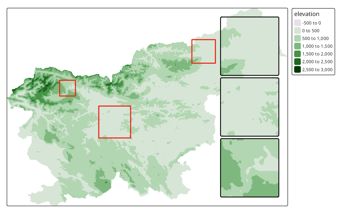
Figure 15.1 shows how to add multiple inset maps to a main map. Each inset is defined by a bounding box using the tmaptools::bb() function, which takes a place name as input and returns a bounding box for that place.1 In such cases, inset maps are added to the main map, with the same extent as the bounding box and the same style as the main map.
The above map can be further customized by improving the color palette and adding titles to the inset maps. We can use the tm_title() function to add titles to the inset maps, and the tm_inset() function to specify the bounding boxes for each inset map. Then, each of these components can be grouped using the group_id argument and arranged using the tm_components() function (Section 11.2).
tm_shape(slo_elev) +
  tm_raster(
    col.scale = tm_scale_continuous(values = "geyser", midpoint = NA)
  ) +
  tm_title("Maribor", group_id = 1) +
  tm_inset(tmaptools::bb("Maribor"), group_id = 1) +
  tm_title("Ljubljana", group_id = 1) +
  tm_inset(tmaptools::bb("Ljubljana"), group_id = 1) +
  tm_title("Bled", group_id = 2) +
  tm_inset(tmaptools::bb("Bled"), group_id = 2) +
  tm_components(1, position = c("right", "bottom")) +
  tm_components(2, position = c("left", "top"))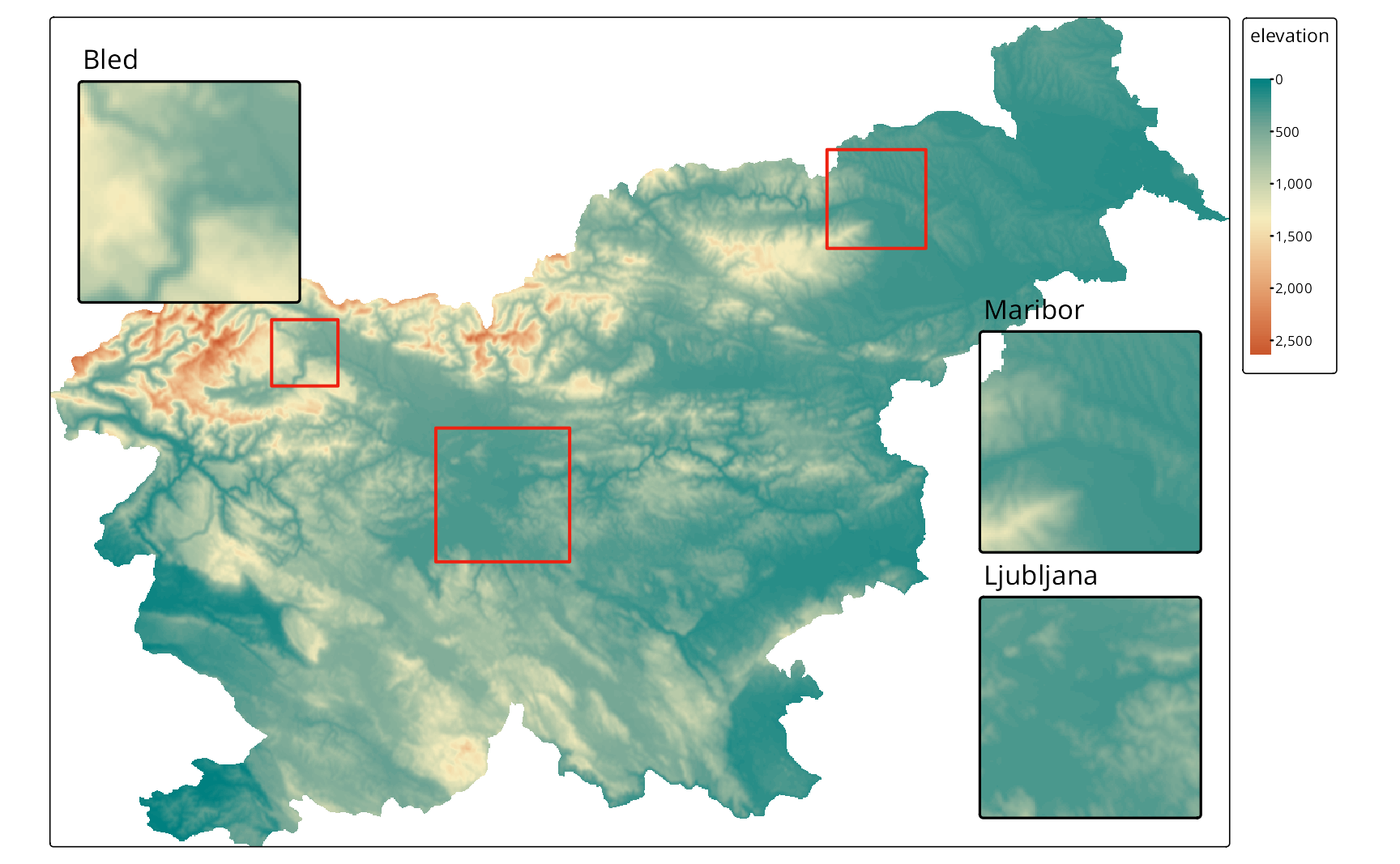
The tm_inset() function can also be used to add a tmap object as an inset map. In the following example, we create a tmap object for Slovenia’s elevation. Importantly, we set the limits of the color scale to match the limits of the elevation data of the main map and remove the legend using the tm_legend(show = FALSE) argument to avoid duplication of the legend in the inset map. We also add a scale bar to the inset map using the tm_scalebar() function to facilitate a better understanding of the area’s size shown in the inset.
tm_slo_elev = tm_shape(slo_elev) +
  tm_raster(
    col.scale = tm_scale_continuous(values = "geyser", midpoint = NA,
                                    limits = c(-100, 4000)),
    col.legend = tm_legend(show = FALSE)
  ) +
  tm_scalebar(breaks = c(0, 10, 20),
              position = c("RIGHT", "BOTTOM"))
Now, we can create our main map and add the inset map based on the tm_slo_elev object (Figure 15.3). The main map in our case would be the elevation of Europe, using the same color scale as the inset map – however, this time, we include the legend.
worldelevation = rast("data/worldelevation.tif")
tm_shape(worldelevation, bbox = "Europe") +
  tm_raster(
    col.scale = tm_scale_continuous(values = "geyser", midpoint = NA,
                                    limits = c(-100, 4000))
  ) +
  tm_scalebar() +
  tm_title("Slovenia", group_id = 1) +
  tm_inset(tm_slo_elev, group_id = 1) +
tm_components(1, position = c("LEFT", "TOP")) 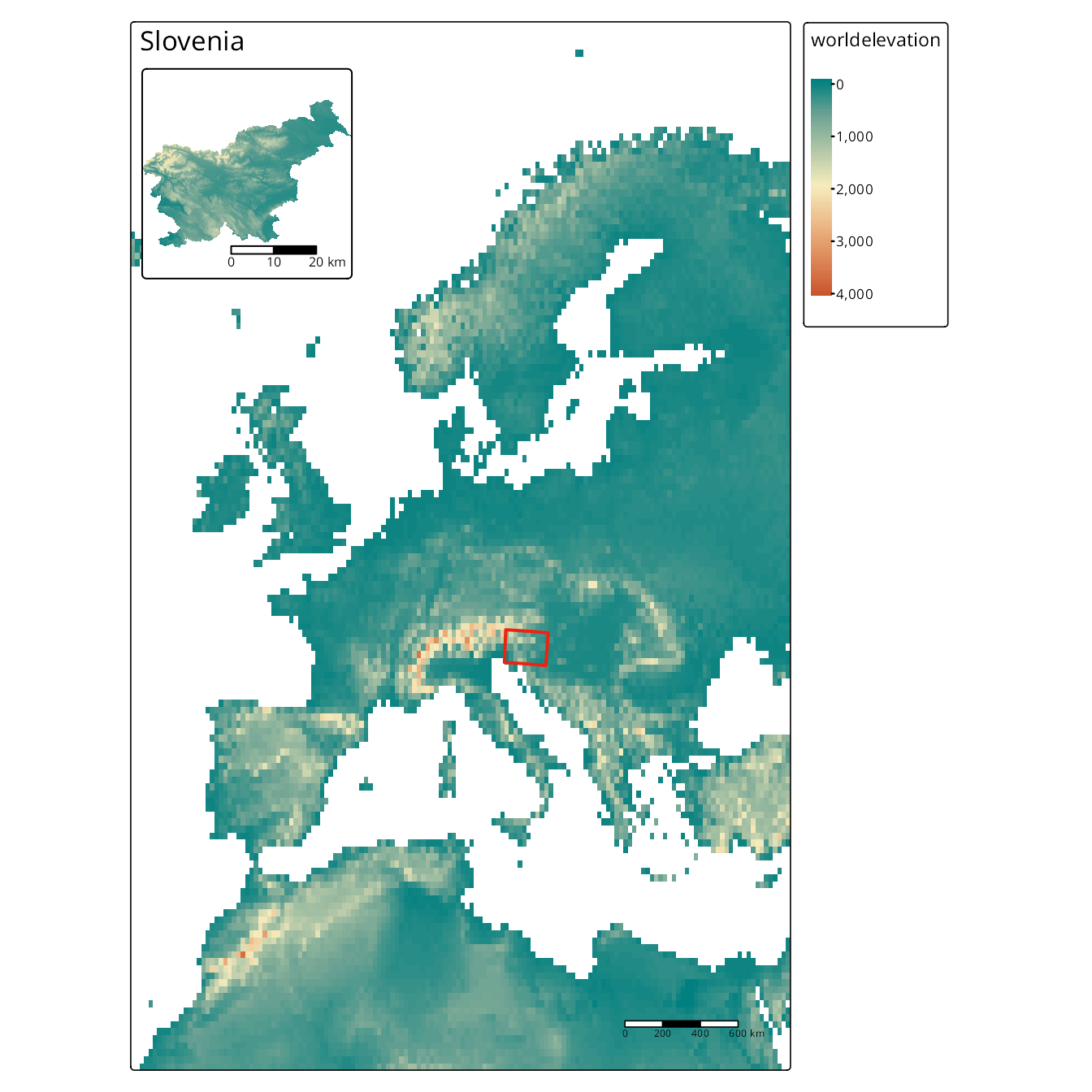
The ggplot2 package can also be used to create insets. Such insets could be based on some external data or be derived from the map data itself to provide additional non-spatial information. In the following example, we create a bar plot illustrating the number of people living in Slovenia’s cities and towns. The default ggplot2 theme includes many elements, such as grid lines, axis ticks, and background, which are often unnecessary in inset maps and can distract from the main map. Thus, we also remove the labeling of the axes and apply the theme_minimal() function to simplify the plot.
We can add the new ggplot2 object as an inset map in the same way as we did with the tmap object. Figure 15.4 displays a map of Slovenia’s regions, with points representing cities and towns, and then adds the ggplot2 object as an inset map. It allows us to see that even though there are more towns than cities in our dataset, more people live in cities than in towns.
slo_regions = read_sf("data/slovenia/slo_regions.gpkg")
tm_shape(slo_regions) +
  tm_polygons("gdppercap") +
  tm_shape(slo_cities) +
  tm_symbols(shape = "place") +
  tm_labels("name", bgcol = "white") +
tm_inset(gg1, position = c("right", "bottom")) 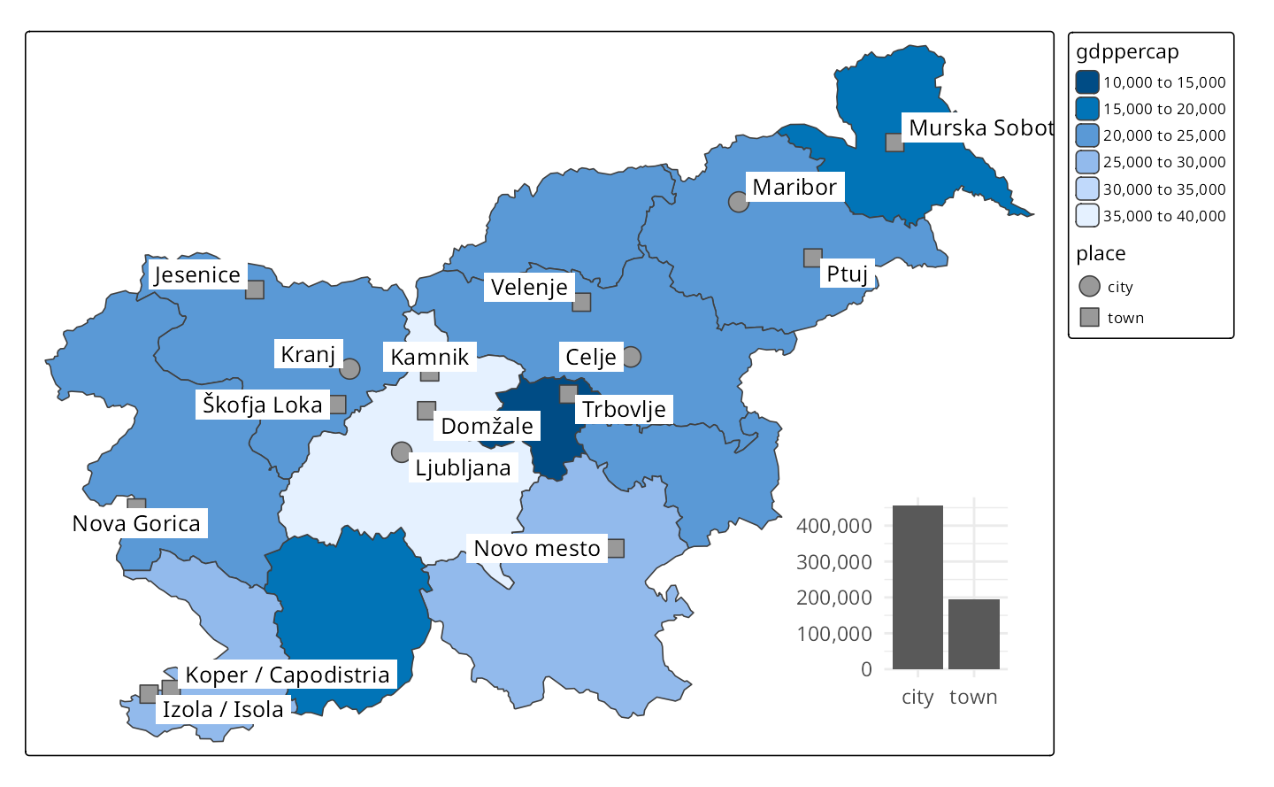
Note
Insets are not usually needed in the interactive mode, as we can zoom in and out of the main map. Thus, the tm_inset() function calls only work in plot mode.
15.2 Basic arrangements
Let’s see how the tmap_arrange() function works based on two maps of Slovenia, each based on different data sources. The first map is based on the GDP per capita of Slovenia’s regions, represented as polygons.
The second map is based on the elevation of Slovenia, represented as a raster layer.
In both cases, we also added titles to the maps using the tm_title() function to clarify what each map represents, and assigned them to the objects tm1 and tm2. Now, we may arrange these two maps in a single layout using the tmap_arrange() function (Figure 15.5). The tmap_arrange() function can take any number of tmap objects as input or even a list of tmap objects.
tmap_arrange(tm1, tm2, ncol = 2)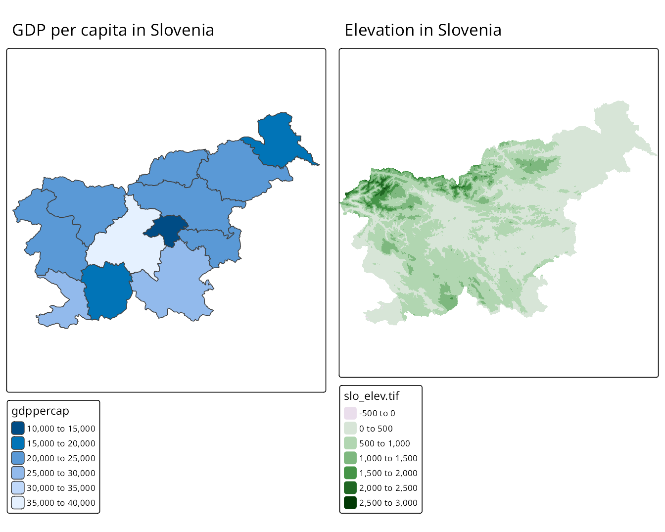
In the example above, we used our two maps and specified the number of columns in the layout using the ncol argument. We can also specify the number of rows using the nrow argument, the aspect ratio of the maps using the asp argument, and the widths and heights of the maps using the widths and heights arguments, respectively.
15.3 Customizing arrangements
The tmap_arrange() does not align layouts of multiple maps – you may notice that the frames of the two maps in Figure 15.5 are not equal in height. To align the frames of the maps, we can use the meta.margins argument in the tm_layout() function for each map. This argument allows us to specify the margins around the map frame available for map elements, such as titles and legends, in the order of c(bottom, left, top, right).
Here, we set the bottom margin to 0.3 for both maps, which will align their frames vertically. See the effect of this change in Figure 15.6.
tm1a = tm1 +
  tm_layout(meta.margins = c(0.3, 0, 0, 0))
tm2a = tm2 +
  tm_layout(meta.margins = c(0.3, 0, 0, 0))
tmap_arrange(tm1a, tm2a, ncol = 2)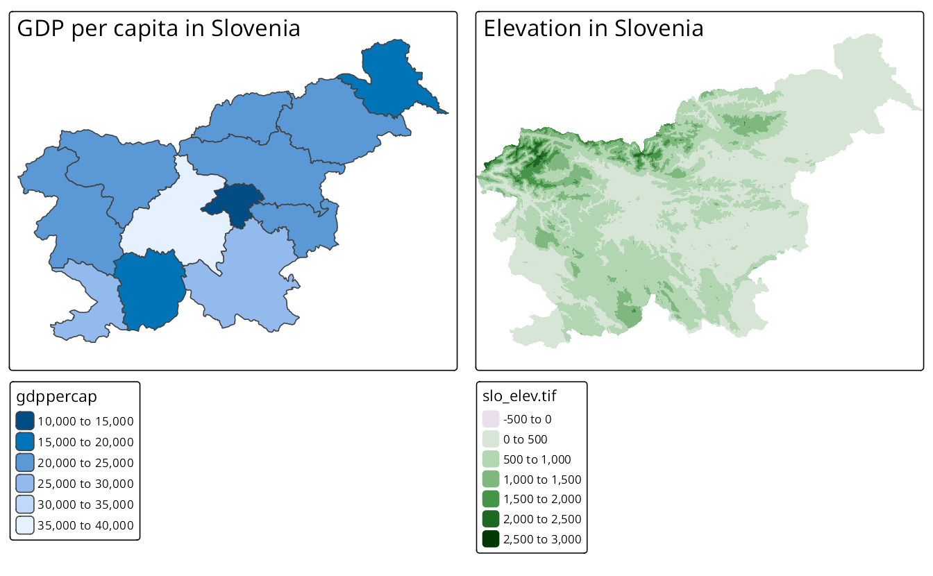
You may also notice that, as we set the top margin of the second map to 0, the titles of both maps were moved inside the map frames. If you want to keep the titles outside, you can set the top margin of the second map to a small value, such as 0.05.
Note
The outcomes of the tmap_arrange() function also work in the tmap view mode, which allows you to explore a few maps at once interactively.
Note
The tmap_arrange() function call can be saved to an object, which can then be used in other functions, such as tmap_save(), to save the arranged maps to a file. For more information on saving maps, see Chapter 4.
Alternatively, you can use a bounding box defined by a vector of coordinates, such as
c(xmin, ymin, xmax, ymax)or another spatial object.↩︎