13 Map projections
This chapter gives a background on why do we need map projections and how to translate spatial data from an ellipsoid into a flat surface or computer screen. Then, it explains basic terms, gives an overview of map projections, and provides guidelines for choosing a suitable map projection for a specific application. Finally, it shows how to use R and the tmap package to specify and customize map projections.
13.1 What are map projections?
We use maps so often in everyday life that most of us probably forget that a map is just a two-dimensional representation of a three-dimensional object, namely the Earth. For centuries, geographers and mathematicians wondered what the best way is to do this. Let us wonder with them for a second.
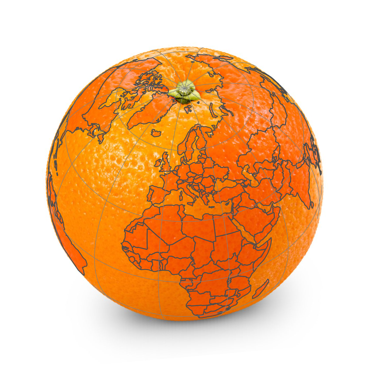
The world is depicted as an orange in Figure 13.1, not just to stimulate your appetite for this subject, but also because an orange peel serves as a good analogy for a two-dimensional map. A world map can be seen as an orange peel laid out on the table. The question is how to peel the orange and how to put the peel flat on the table.
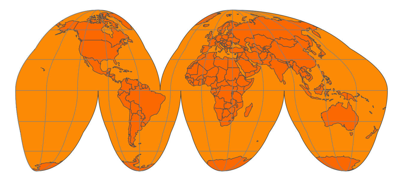
When we peel the orange, ideally, we want to rip the peel near areas of the Earth that are less interesting. What is interesting depends on the application – for applications where land mass is more important than water mass, it is a good idea to make the rips in the oceans. The (interrupted) Goode homolosine projection (Figure 13.2) embodies this idea. All continents and countries are preserved except Antarctica and Greenland. There is also a version of the Goode homolosine projection that focuses on preserving the oceans.
To make the analogy between the orange peel and the surface of the Earth complete, we have to assign two fictitious properties to the orange peel, namely that it is stretchable and deformable. These properties are needed in order to make a non-interrupted map, as we will see in the following sections.
A method to flatten down the Earth, for which the Goode homolosine projection shown in Figure 13.2 is an example, is called a map projection. Technically, it is also known as a coordinate reference system (CRS), which specifies the corresponding coordinate system, as well as the transformations to other map projections.
13.2 A model of the Earth
The orange and the Earth have another thing in common: both are spheres, but not perfect ones. The Earth is metaphorically speaking a little fat: the circumference around the equator is 40,075 km, whereas around the circumference that crosses both poles is 40,009 km. Therefore, the Earth can better be described as an ellipsoid. The same applies to an orange: every orange is a little different, but probably very few oranges are perfect spheres.
Although the ellipsoid is a good mathematical model to describe the Earth’s surface, keep in mind that the surface of the Earth is not smooth – land mass usually lies at a higher altitude than sea level. We could potentially map each point on the surface of the Earth using a three-dimensional \((x, y, z)\) Cartesian coordinate system with the center of the mass of the Earth being the origin (0, 0, 0). However, since this has many mathematical complications, the ellipsoid is often sufficient as a model of the surface of the Earth.
This ellipsoid model and its translation to the Earth’s surface is called a (geodetic) datum. Many datums exist, for global and local applications. The most popular global datum is WGS84, which was introduced in 1984 as an international standard and was last revised in 2004. Then, there are many local datums, which are often tailored for specific regions or countries. For instance, NAD83, ETRS89, and GDA94 are slightly better models for North America, Europe, and Australia, respectively. However, since WGS84 is a very good approximation of the Earth as a whole, it has been widely adopted worldwide and is also used by the Global Positioning System (GPS).
When we have specified a datum, we are able to describe geographic locations with two familiar variables, namely latitude and longitude. The latitude defines the north-south position in degrees, where latitude = 0\(^\circ\) is the equator. The latitudes for the north and south poles are 90\(^\circ\) and \(-90^\circ\), respectively. The longitude specifies the east-west position in degrees, where by convention, the longitude = 0\(^\circ\) meridian crosses the Royal Observatory in Greenwich, UK. The longitude range is -180\(^\circ\) to 180\(^\circ\), and since this is a full circle, -180\(^\circ\) and \(^\circ\) specify the exact longitude.
When we see the Earth in its three-dimensional form, as in Figure 13.1, the latitude parallels are the horizontal lines around the Earth, and the longitude meridians are the vertical lines around the Earth. The set of longitude meridians and latitude parallels is also referred to as graticule. In all the figures in this section, latitude parallels are shown as gray lines for \(-60^\circ\), \(-30^\circ\), \(0^\circ\), \(30^\circ\) and \(60^\circ\), and longitude meridians from \(-180^\circ\) to \(180^\circ\) at every \(30^\circ\).
Please keep in mind that only a latitude and longitude are not sufficient to specify a geographic location. A datum is required. When people exchange latitude-longitude data, it is often safe to assume that they implicitly have used the WGS84 datum. However, it is good practice to specify the datum explicitly.
13.3 Platte Carrée and Web Mercator
Let’s take a closer look at two widely used map projections, namely the plain latitude-longitude coordinate system (using the WGS84 datum) and the Web Mercator projection, which is currently the de facto standard for interactive maps. These projections are indexed as EPSG:4326 and EPSG:3857 respectively. EPSG is a database of standard map projections.
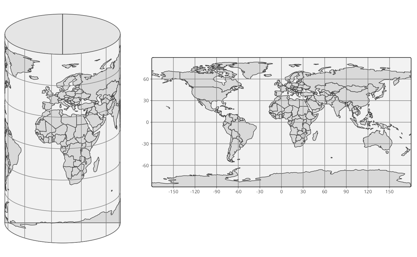
When we fictitiously make little holes in the orange peel at both poles, and stretch these open so wide that they have the same width as the equator, we obtain the cylinder depicted in Figure 13.3 (left). Note that the longitude lines have become straight vertical lines. When we unroll this cylinder, we obtain a map where the \(x\) and \(y\) coordinates are the longitude and latitude, respectively. This CRS, which is known as EPSG:4326, is shown in Figure Figure 13.3 (right).
EPSG:4326 is an unprojected CRS since the longitude and latitude have not been transformed. With projected CRSs, the \(x\) and \(y\) coordinates refer to specific measurement units, usually meters. The projected variant of this CRS is called the Platte Carrée (EPSG:4087), and is exactly the same map as shown in Figure Figure 13.3 (right), but with other \(x\) and \(y\) value ranges.
Observe since we stretched the poles open, the area near the poles has been stretched out as well. More specifically, the closer the land is to one of the poles, the more it has been stretched out. Since the stretching direction is only horizontal, the shapes of the areas have become wider. A good example is Greenland, which is naturally elongated from north to south (as can be seen in Figure 13.1).
In order to fix these deformed areas, Gerardus Mercator, a Flemish geographer in the 16th century, introduced a method to compensate for this by inflating the areas near the poles even more, but now only in a vertical direction. This projection is called the Mercator projection. For web applications, this projection has been slightly modified and renamed to the Web Mercator projection (EPSG:3857). The cylinder and plain map that uses this projection are shown in Figure 13.4.
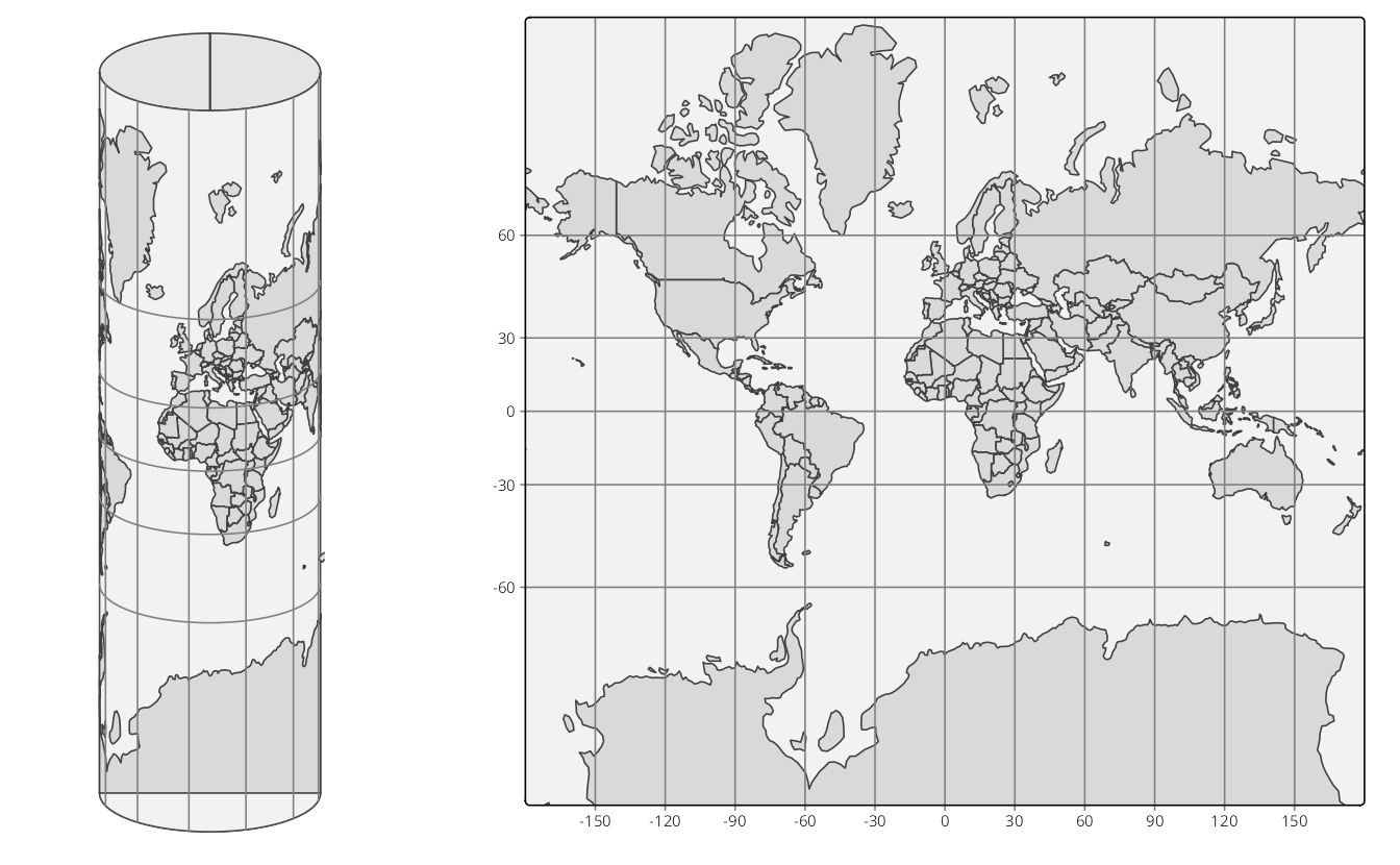
Although the areas near the poles have been inflated quite a lot, especially Antarctica and Greenland, the shape of the areas is more or less correct, in particular regarding small regions (which can be seen by comparing with Figure 13.1). The Mercator projection is very useful for navigational purposes and has therefore been embraced by sailors ever since. Also, today, the Web Mercator is the de facto standard for interactive maps and navigation services. However, for maps that show data, the (Web) Mercator projection should be used with great caution because the hugely inflated areas influence how we perceive spatial data. We discuss this in the next section.
13.4 Types of map projections
Let us return to the original question: how can we create a two-dimensional representation of our three-dimensional Earth? Although there are many ways, four basic map projection types can be distinguished. These are depicted in Figure 13.5.
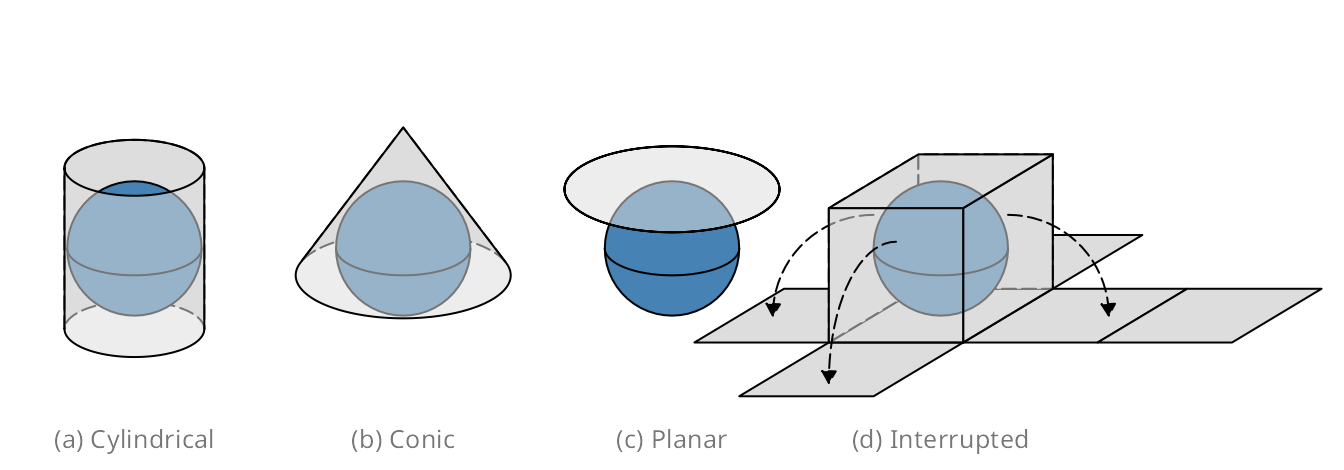
Examples of cylindrical projections have already been given in the previous section: both Platte Carrée and Web Mercator are cylindrical. Another widely used cylindrical map projection is the Universal Transverse Mercator (UTM). Its cylinder is not placed upright but horizontally. There are 60 positions in which this cylinder can be placed, where in each position, the cylinder faces a longitude range of 6 degrees. In other words, the UTM is not a single projection, but a series of 60 projections.
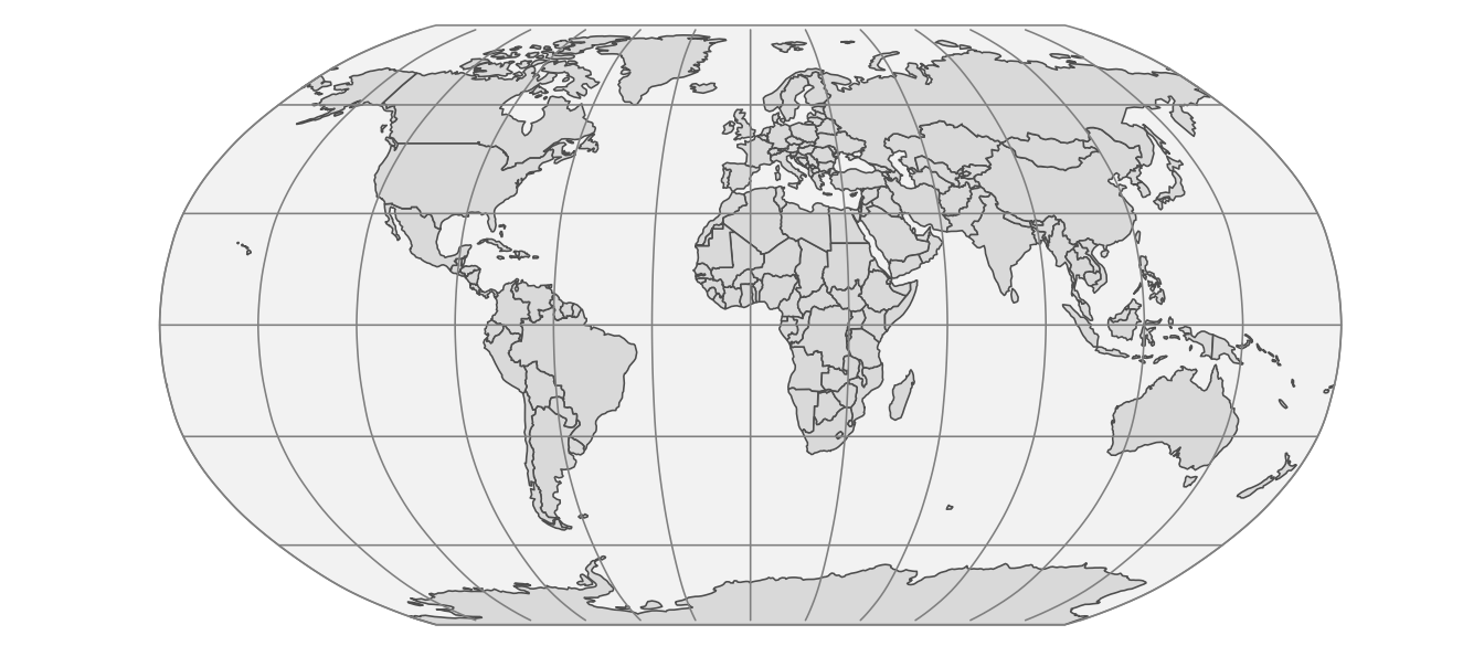
There are many projections that are pseudo-cylinders in the sense that the radius around the poles is smaller than around the equator. An example is the Robinson projection shown in Figure 13.6. Almost all commonly used standard World map projections are (pseudo-)cylindrical.
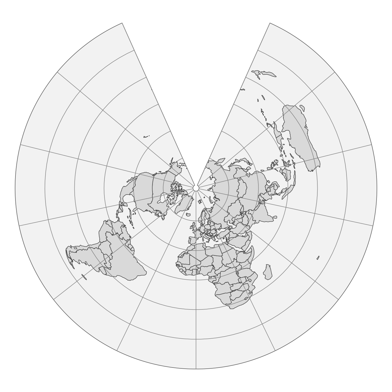
An example of a conic map projection is shown in Figure 13.7 (a). As a result of unfolding a cone on a flat surface, a gap is created. The size (angle) of this gap depends on the width of the cone. There are also pseudo-conic map projections in which some meridians (longitude lines) are curved. Conic map projections are useful for mid-latitude areas where the Earth’s surface and the cone are nearly parallel to each other.
Planar map projections, also known as azimuthal projections, project the Earth on a disk. This can be done in several ways. One effective method is to use the position of an imaginary light source. The light source can be positioned in three different ways: inside the globe, at the surface of the globe opposite the disk, or at an infinite distance from the disk. The corresponding families of projections are called gnomonic, stereographic, and orthogonal projections.
Planar map projections are often used for a specific country or continent. An example is the Lambert Azimuthal Equal-Area projection (EPSG:3035), shown in Figure 13.7 (b), which is optimized for Europe. It can be classified as a stereographic projection, although the light beams are not straight but curved. Another example of a planar map projection is the orange shown in Figure 13.1. This is an orthogonal projection.
The (interrupted) Goode homolosine projection shown in Figure 13.2 is an example of an interrupted projection. A special class of these projections are polyhedral projections, which consist of planar faces. In Figure 13.5 a polyhedral of six faces is illustrated. There is no limit to the number of faces, as the myriahedral projections illustrate.
13.5 Which projection to choose?
Hopefully, it is clear that there is no perfect projection, as each has its pros and cons. Whether a projection is suitable for a certain application depends on two factors. The first factor is the type of application and, in particular, which map projection properties are useful or even required for that application (Section 13.5.1). For instance, navigation requires other map projection properties than statistical maps. The second factor is the area of interest (Section 13.5.2). Is the whole World visualized or only a part, and in the latter case, which part? In this section, guidelines are provided to help you choose a suitable projection based on these two aspects.
Before we delve deeper into selecting a projection, it is worth noting that for many countries and continents, government agencies have already chosen projections to be the standard for mapping spatial data. For instance, a standard for Europe, used by Eurostat (the statistical agency of the European Union), is the Lambert Azimuthal Equal-Area projection, shown in Figure 13.7 (b). If the area of interest has such a standard, it is recommended to use it, because it can be safely assumed that this standard is a proper projection, and moreover, it makes cooperation and communication with other parties easier. However, be aware of the limitations that this particular projection may have, and that there may be better alternatives out there.
13.5.1 Map projection properties
The type of application is important for the choice of a map projection. However, it would be quite tedious to list all possible applications and provide projection recommendations for each of them. Instead, we focus on four map projection properties. The key step is to find out which of these properties are useful or even required for the target application. The four properties are listed in Table 13.1.
| Property | Conformal | Equal area | Equidistant | Azimuthal |
| Preserves | Local angle (shape) | Area | Distance | Direction |
| Applications | Navigation, climate | Statistics | Geology | Geology |
| Examples (cyclindrical) | Mercator | Gall-Peters, Eckert IV | Equirectangular | none |
| Examples (conic) | Lambert conformal conic | Albers conic | Equidistant conic | none |
| Examples (planar) | Stereographic | Lambert azimuthal equal-area | Azimuthal equidistant | Stereographic, Lambert azimuthal equal-area |
| Examples (interrupted) | Myriahedral | Goode homolosine, Myriahedral | none | none |
A conformal projection means that local angles are preserved. In practice, that means, for instance, that a map of a crossroad preserves the angles between the roads. Therefore, this property is required for navigational purposes. As a consequence, local angles are preserved, and local shapes are also preserved. That means that a small island are drawn on a map in its true shape, as seen from the sky perpendicular above it. The Web Mercator, as shown in Figure 13.4, satisfies this property. The closer an area is to one of the poles, the more it is enlarged, but since this is done in both dimensions (latitude and longitude), local shapes are preserved.
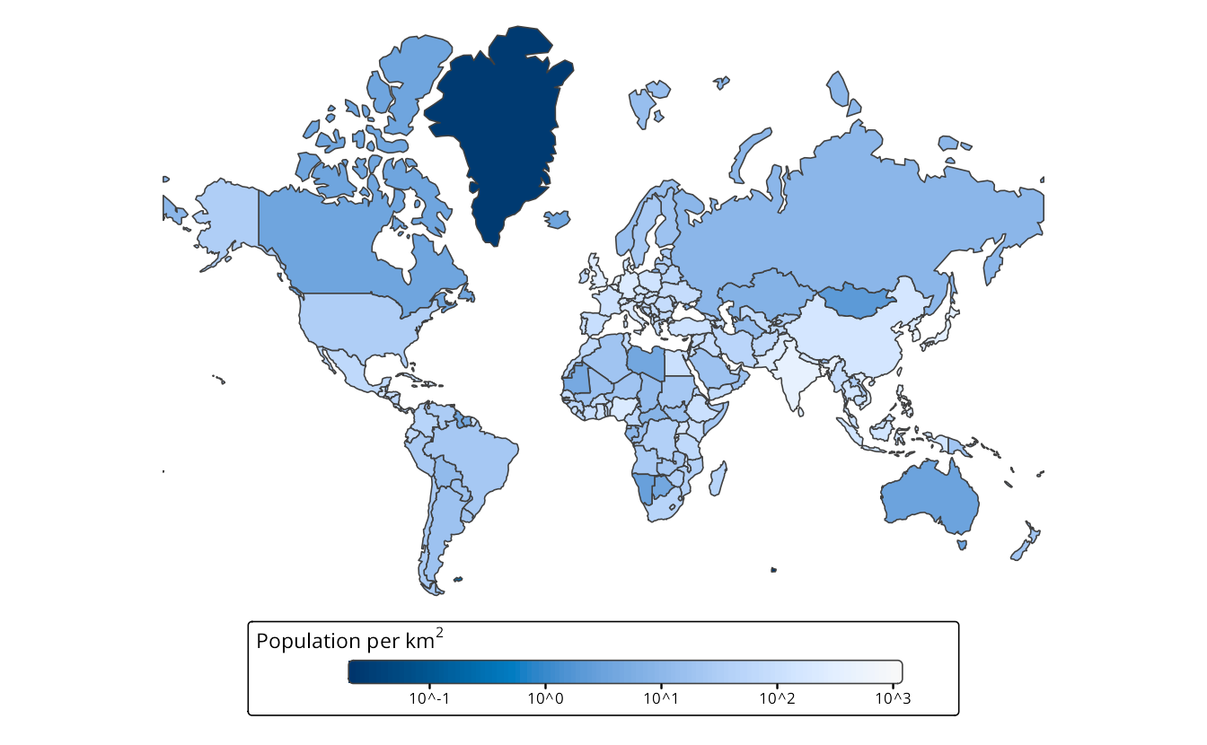
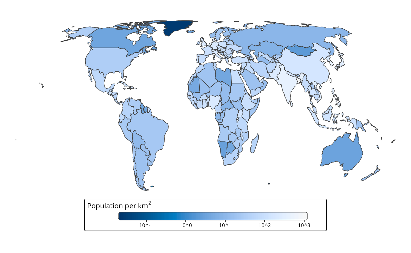
A map projection is called equal-area if the areas are proportional to the true areas. This is strongly recommended for maps that display statistics to prevent perceptual bias. Figure 13.8 shows two World maps of population density per country, one in the Web Mercator projection and the other in Eckert IV projection. The perception of the World population is different in these maps – in (a) the vast lands in low-populated areas seem to be Canada, Greenland, and Russia, whereas in (b) also North Africa and Australia emerge as vast low-populated areas.
The other two map projection properties are related to one central point on the map. A map projection is called equidistant if the distances to any other point in the map are preserved and azimuthal if the directions to any other point are preserved. These properties are, in particular, useful in the field of geology. One example is a seismic map around the epicenter of a recent earthquake, where it is crucial to show how far and in which direction the vibrations are spreading.
A map projection can satisfy at most two of these properties. Many map projections do not fulfill any property but are intended as a compromise. An example is the Robinson projection, shown in Figure 13.6.
13.5.2 Area of interest
The next aspect that is important for the choice of a map projection is the area of interest. In general, the larger the area, the more concessions have to be made, since the larger the area, the more difficult it is to create a two-dimensional projection.
The following Table 13.2 provides recommendations for map projection types based on the area size and latitude of the area.
| View | Low latitude (equator) | Mid latitude | High latitude (poles) |
|---|---|---|---|
| World | Pseudo-cylindrical | Pseudo-cylindrical | Pseudo-cylindrical |
| Hemisphere | Azimuthal | Azimuthal | Azimuthal |
| Continent or smaller | Cylindrical or azimuthal | Conic or azimuthal | Azimuthal |
For World maps, pseudo-cylindrical map projections, such as the Robinson projection (Figure 13.6) and the Eckert IV projection (Figure 13.8 (b)) are very popular because they have less distortion than other map projections. For areas that cover half of the sphere, i.e., a hemisphere, azimuthal map projections are recommended. Four hemispheres are often used: the Northern and Southern Hemispheres, with the North and South Poles as their centers, the Western Hemisphere consisting of the Americas, and the Eastern Hemisphere, which includes the other continents. However, other hemispheres are often used implicitly, such as a hemisphere centered on Europe used in the Lambert Azimuthal Equal-Area projection shown in Figure 13.7 (b).
For areas with the size of a continent or country, the azimuthal map projection type can be used when centered on the area of interest. In particular, the Lambert Azimuthal Equal-Area projection is used when equal area is required, and the Azimuthal Equidistant projection is used when preserving distances is essential. Alternatively, cylindrical and conic map projection types can be used for areas at low and mid-latitudes, respectively. Another alternative is to use a UTM projection. However, this is only recommended when the target area spans less than 6 degrees longitude and does not cross the UTM zone lines.
13.6 CRS in R
Coordinate Reference Systems (CRSs) are implemented in the software library PROJ. With implementation, we mean specifying a CRS and transforming coordinates from one CRS to another. PROJ is used by every popular software application for spatial data, in particular, ArcGIS, QGIS, and GRASS GIS, and also by many programming languages, including R. The sf and terra packages integrate the PROJ capabilities into R.
A CRS is represented in sf by an object of class crs, which can be retrieved or set with the function st_crs(). In the following example, a crs object is created from an EPSG code, in this case, 3035, the Lambert Azimuthal Equal-Area projection for Europe.
library(sf)
# CRS Lambert Azimuthal Equal-Area projection
st_crs("EPSG:3035")
#> Coordinate Reference System:
#>   User input: EPSG:3035
#>   wkt:
#> PROJCRS["ETRS89-extended / LAEA Europe",
#>     BASEGEOGCRS["ETRS89",
#>         ENSEMBLE["European Terrestrial Reference System 1989 ensemble",
#>             MEMBER["European Terrestrial Reference Frame 1989"],
#>             MEMBER["European Terrestrial Reference Frame 1990"],
#>             MEMBER["European Terrestrial Reference Frame 1991"],
#>             MEMBER["European Terrestrial Reference Frame 1992"],
#>             MEMBER["European Terrestrial Reference Frame 1993"],
#>             MEMBER["European Terrestrial Reference Frame 1994"],
#>             MEMBER["European Terrestrial Reference Frame 1996"],
#>             MEMBER["European Terrestrial Reference Frame 1997"],
#>             MEMBER["European Terrestrial Reference Frame 2000"],
#>             MEMBER["European Terrestrial Reference Frame 2005"],
#>             MEMBER["European Terrestrial Reference Frame 2014"],
#>             MEMBER["European Terrestrial Reference Frame 2020"],
#>             ELLIPSOID["GRS 1980",6378137,298.257222101,
#>                 LENGTHUNIT["metre",1]],
#>             ENSEMBLEACCURACY[0.1]],
#>         PRIMEM["Greenwich",0,
#>             ANGLEUNIT["degree",0.0174532925199433]],
#>         ID["EPSG",4258]],
#>     CONVERSION["Europe Equal Area 2001",
#>         METHOD["Lambert Azimuthal Equal Area",
#>             ID["EPSG",9820]],
#>         PARAMETER["Latitude of natural origin",52,
#>             ANGLEUNIT["degree",0.0174532925199433],
#>             ID["EPSG",8801]],
#>         PARAMETER["Longitude of natural origin",10,
#>             ANGLEUNIT["degree",0.0174532925199433],
#>             ID["EPSG",8802]],
#>         PARAMETER["False easting",4321000,
#>             LENGTHUNIT["metre",1],
#>             ID["EPSG",8806]],
#>         PARAMETER["False northing",3210000,
#>             LENGTHUNIT["metre",1],
#>             ID["EPSG",8807]]],
#>     CS[Cartesian,2],
#>         AXIS["northing (Y)",north,
#>             ORDER[1],
#>             LENGTHUNIT["metre",1]],
#>         AXIS["easting (X)",east,
#>             ORDER[2],
#>             LENGTHUNIT["metre",1]],
#>     USAGE[
#>         SCOPE["Statistical analysis."],
#>         AREA["Europe - European Union (EU) countries and candidates. Europe - onshore and offshore: Albania; Andorra; Austria; Belgium; Bosnia and Herzegovina; Bulgaria; Croatia; Cyprus; Czechia; Denmark; Estonia; Faroe Islands; Finland; France; Germany; Gibraltar; Greece; Hungary; Iceland; Ireland; Italy; Kosovo; Latvia; Liechtenstein; Lithuania; Luxembourg; Malta; Monaco; Montenegro; Netherlands; North Macedonia; Norway including Svalbard and Jan Mayen; Poland; Portugal including Madeira and Azores; Romania; San Marino; Serbia; Slovakia; Slovenia; Spain including Canary Islands; Sweden; Switzerland; Türkiye (Turkey); United Kingdom (UK) including Channel Islands and Isle of Man; Vatican City State."],
#>         BBOX[24.6,-35.58,84.73,44.83]],
#>     ID["EPSG",3035]]
A crs object contains Well Known Text (WKT). It includes a specification of the used datum as well as information on how to transform it into other CRSs. Understanding the exact content of the WTK is not important for most users, since it is not needed to write a WKT yourself.
A crs object can be created in several ways:
- The first is with an EPSG number as a user input specification, as shown above.
- The second is also with a user input specification, but with a so-called proj4 character string. The proj4 character string for the LAEA projection is
"+proj=laea +lat_0=52 +lon_0=10 +x_0=4321000 +y_0=3210000 +ellps=GRS80 +units=m +no_defs". However, proj4 character strings should be used with caution since they often lack important CRS information regarding datums and CRS transformations. Also note that the name proj4 stands for the PROJ library version 4, while the current major version of PROJ at the time of writing is already 9. - The third way is to provide a WKT definition of the projection.
- The last way to create a
crsobject is to extract it from an existing spatial data object (e.g., an sf, terra, or stars object) using thest_crs()function.
A crs object can define a new spatial object’s projection or transform an existing spatial object into another projection. In the example below, we created a new object, waterfalls, with names and coordinates of three famous waterfalls. Next, we converted it into a spatial object of the sf class, waterfalls_sf() with st_as_sf(). We can see that our object’s coordinate reference system is not defined with the st_crs() function.
# create a data frame of three famous waterfalls
waterfalls = data.frame(name = c("Iguazu Falls", "Niagara Falls", "Victoria Falls"),
                        lat = c(-25.686785, 43.092461, -17.931805),
                        lon = c(-54.444981, -79.047150, 25.825558))
# create sf object (without specifying the crs)
waterfalls_sf = st_as_sf(waterfalls, coords = c("lon", "lat"))
# extract crs (not defined yet)
st_crs(waterfalls_sf)
#> Coordinate Reference System: NA
This function also allows us to specify CRS of our object – in this example, coordinates of our object are in the WGS84 coordinate system, and thus we can use the EPSG code of 4326. We can also confirmed that our operation was successful also using st_crs().
# specify crs
st_crs(waterfalls_sf) = "EPSG:4326"
# extract crs
st_crs(waterfalls_sf)
#> Coordinate Reference System:
#>   User input: EPSG:4326
#>   wkt:
#> GEOGCRS["WGS 84",
#>     ENSEMBLE["World Geodetic System 1984 ensemble",
#>         MEMBER["World Geodetic System 1984 (Transit)"],
#>         MEMBER["World Geodetic System 1984 (G730)"],
#>         MEMBER["World Geodetic System 1984 (G873)"],
#>         MEMBER["World Geodetic System 1984 (G1150)"],
#>         MEMBER["World Geodetic System 1984 (G1674)"],
#>         MEMBER["World Geodetic System 1984 (G1762)"],
#>         MEMBER["World Geodetic System 1984 (G2139)"],
#>         MEMBER["World Geodetic System 1984 (G2296)"],
#>         ELLIPSOID["WGS 84",6378137,298.257223563,
#>             LENGTHUNIT["metre",1]],
#>         ENSEMBLEACCURACY[2.0]],
#>     PRIMEM["Greenwich",0,
#>         ANGLEUNIT["degree",0.0174532925199433]],
#>     CS[ellipsoidal,2],
#>         AXIS["geodetic latitude (Lat)",north,
#>             ORDER[1],
#>             ANGLEUNIT["degree",0.0174532925199433]],
#>         AXIS["geodetic longitude (Lon)",east,
#>             ORDER[2],
#>             ANGLEUNIT["degree",0.0174532925199433]],
#>     USAGE[
#>         SCOPE["Horizontal component of 3D system."],
#>         AREA["World."],
#>         BBOX[-90,-180,90,180]],
#>     ID["EPSG",4326]]
Alternatively, it is possible to set the CRS when creating a new sf object, as you can see below.
The st_transform() function is used to convert the existing vector spatial object’s coordinates into another projection. For example, let’s transform our waterfalls_sf object to the Equal Earth projection (EPSG:8857).
waterfalls_sf_trans = st_transform(waterfalls_sf, "EPSG:8857")
waterfalls_sf_trans
#> Simple feature collection with 3 features and 1 field
#> Geometry type: POINT
#> Dimension:     XY
#> Bounding box:  xmin: -6580000 ymin: -3240000 xmax: 2420000 ymax: 5260000
#> Projected CRS: WGS 84 / Equal Earth Greenwich
#>             name                  geometry
#> 1   Iguazu Falls POINT (-4969711 -3244138)
#> 2  Niagara Falls  POINT (-6583123 5261565)
#> 3 Victoria Falls  POINT (2416945 -2285044)
Figure 13.9 shows the example data in the WGS84 coordinate system on the top and in the Equal Earth projection on the bottom. You can see here that the decision of the projection used has an impact not only on the coordinates (notice the grid values), but also on the continents’ shapes.
13.7 Specifying map projections within tmap
Now that the concepts of map projections are established, we can examine how to specify map projections in tmap. Here, we expand on the short introduction from Section 5.4 and show how to use various tools available in the tm_crs() function.
13.7.1 Vector data
First, see how to specify a map projection for vector data. We use the worldvector.gpkg and worldcities.gpkg datasets – the first one uses the Equal Earth projection (EPSG:8857), and the second one uses the WGS 84 coordinate system (EPSG:4326). Additionally, to show the effect of map projections, we transform the worldvector data into the WGS 84 coordinate system, namely worldvector_wgs84.
Figure 13.10 (a) shows the map of the world in the WGS 84 coordinate system created with the code below. We often see this coordinate system used in various global maps. However, as discussed earlier in this chapter, it is not the best choice for visualizing the whole World – WGS 84 is an unprojected coordinate system, and thus it has a lot of distortions, especially going further from the equator.
tm = tm_shape(worldvector_wgs84) +
tm_polygons() +
tm_shape(worldcities) +
tm_dots() +
tm_text("name")
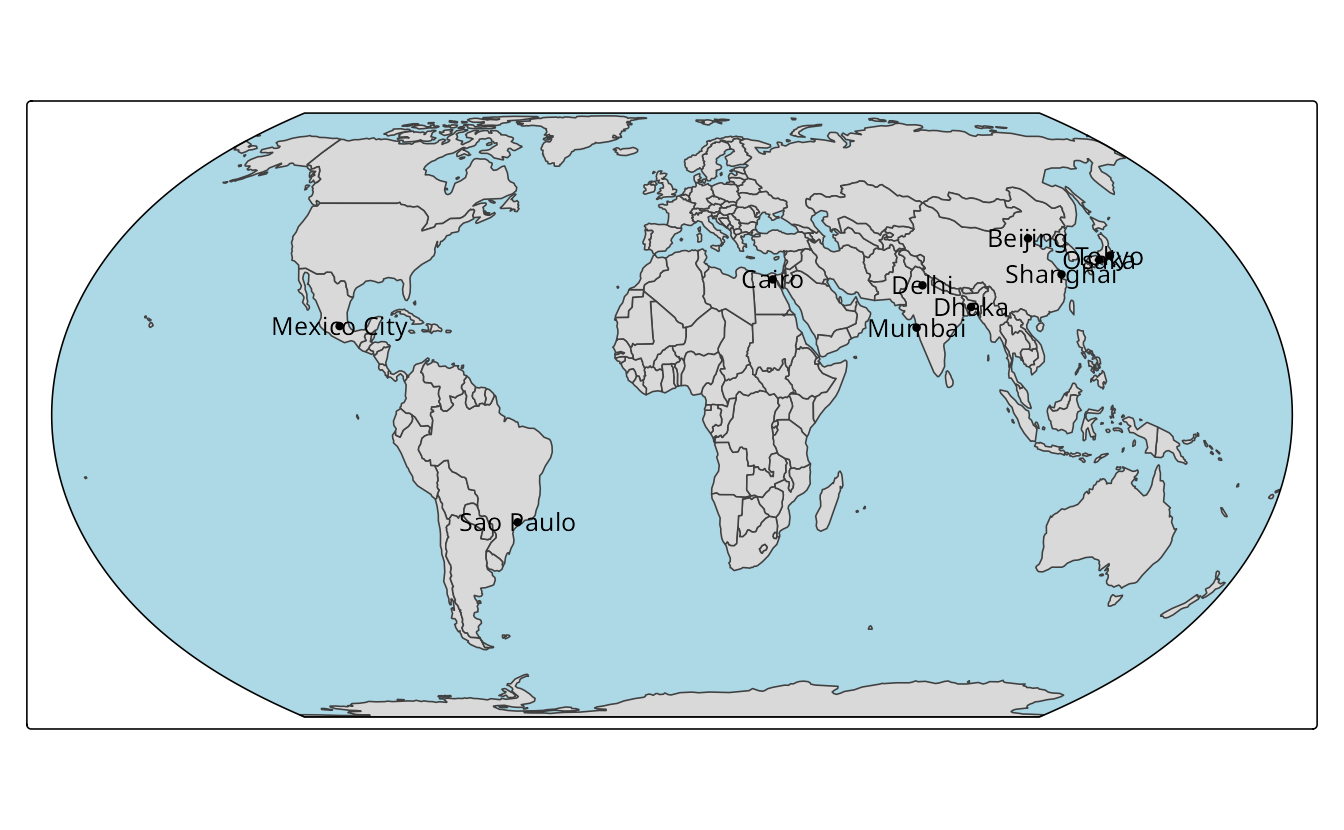
tmWe can improve this map by changing the projection to a more suitable one, such as Equal Earth, directly in the map creation code (Figure 13.10 (b)). We just need to add the tm_crs() function with the desired projection, e.g., tm_crs("+proj=eqearth").
tm +
  tm_crs("+proj=eqearth") # or "EPSG:8857"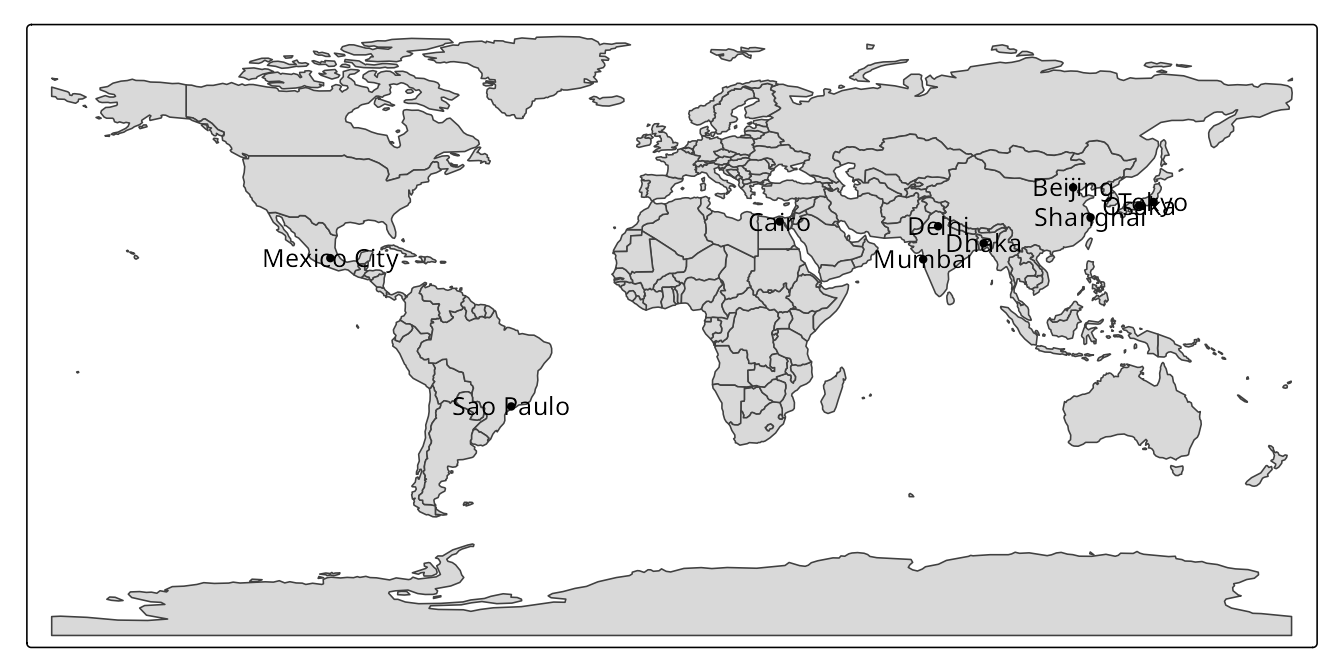

The tm_crs() function is actually a small toolbox for managing map projections. As you have seen above, if we know the projection’s name ("+proj=eqearth") or code ("EPSG:8857") we can specify it directly. You can also use the tm_crs() function if you do not know the projection’s name or code – it accepts the "auto" argument. It automatically select a suitable projection based on the data’s extent and the map’s properties. For example, if the map is global, it selects the pseudocylindrical projection Equal Earth (Figure 13.11).
tm +
  tm_crs("auto")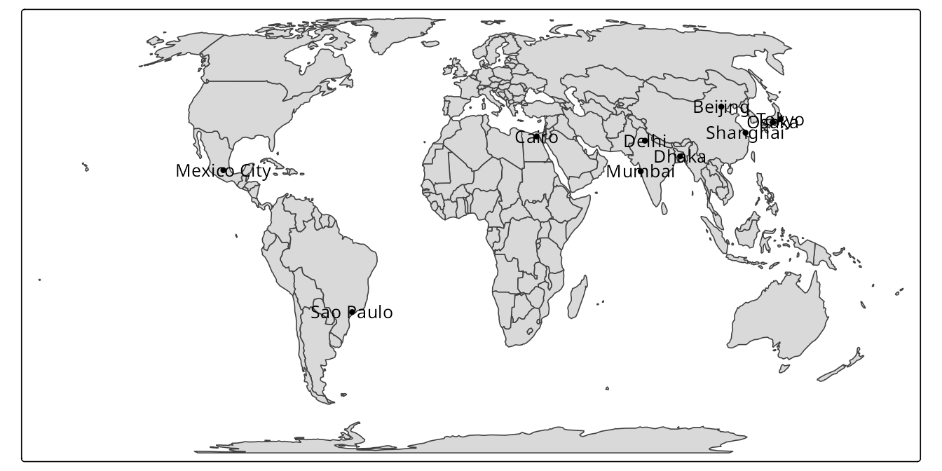
With the tm_crs() function set to "auto", we may also specify the map projection property, such as "area", "distance", or "shape". The "area" property (equal area) uses the Lambert Azimuthal Equal Area projection, "distance" (equidistant) uses the Azimuthal Equidistant projection, and "shape" (conformal) uses the Stereographic projection. Figure 13.12 displays the map with the "distance" property – this means that our data is projected into the Azimuthal Equidistant projection, in this case, with the center on the coordinates of zero latitude and zero longitude. Then, every point on the map is equidistant from that center.
13.7.2 Raster data
The above features of the tm_crs() function also apply to raster data. However, at the same time, reprojecting raster data is more complex than reprojecting vector data. Reprojections of vector data are usually straightforward because each spatial coordinate is reprojected individually. Reprojecting of raster data, on the other hand, is more complex and requires using one of two approaches. The first approach applies raster warping, which is a name for two separate spatial operations: the creation of a new regular raster object and the computation of new pixel values through resampling (for more details, read Chapter 7 of Lovelace et al. (2025)). This is the default option in tmap; however, it has some limitations, and it is not always possible to use it. The second approach involves transforming the coordinates of the raster cells, resulting in a curvilinear grid. Let’s see how to use these two approaches in tmap based on the worldelevation.tif raster data.
Figure 13.13 (a) shows the World elevation raster reprojected to Equal Earth. Some of you can quickly notice that certain areas, such as parts of Antarctica, New Zealand, Alaska, and the Kamchatka Peninsula, are presented twice, with one version being largely distorted. Another limitation of raster.warp = TRUE is the use of the nearest neighbor resampling only – while it can be a proper method to use for categorical rasters, it can have some unintended consequences for continuous rasters (such as the "worldelevation.tif" data).
tm_shape(worldelevation) +
  tm_raster(col.scale = tm_scale(values = terrain.colors(8))) +
  tm_crs("+proj=eqearth") # or "EPSG:8857"
The second approach (tm_options(raster.warp = FALSE)) computes new coordinates for each raster cell, keeping all of the original values, and results in a curvilinear grid. This calculation could deform the shapes of original grid cells, and usually curvilinear grids take a longer time to plot1.
Figure 13.13 (b) illustrates an example of the second approach, which yielded a better result in this case without any spurious land. However, the creation of the (b) map takes about ten times longer than the (a) map.
tm_shape(worldelevation) +
  tm_raster(col.scale = tm_scale(values = terrain.colors(8))) +
  tm_crs("+proj=eqearth") +
  tm_options(raster.warp = FALSE)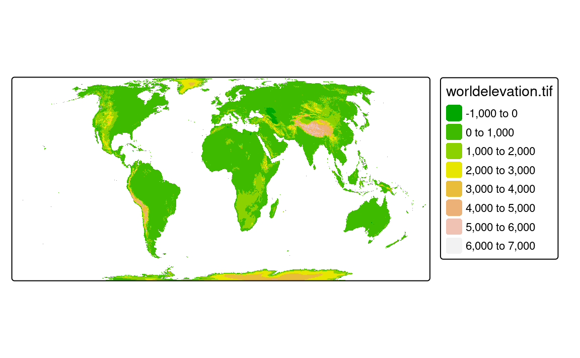

13.8 Customizing maps for global projections
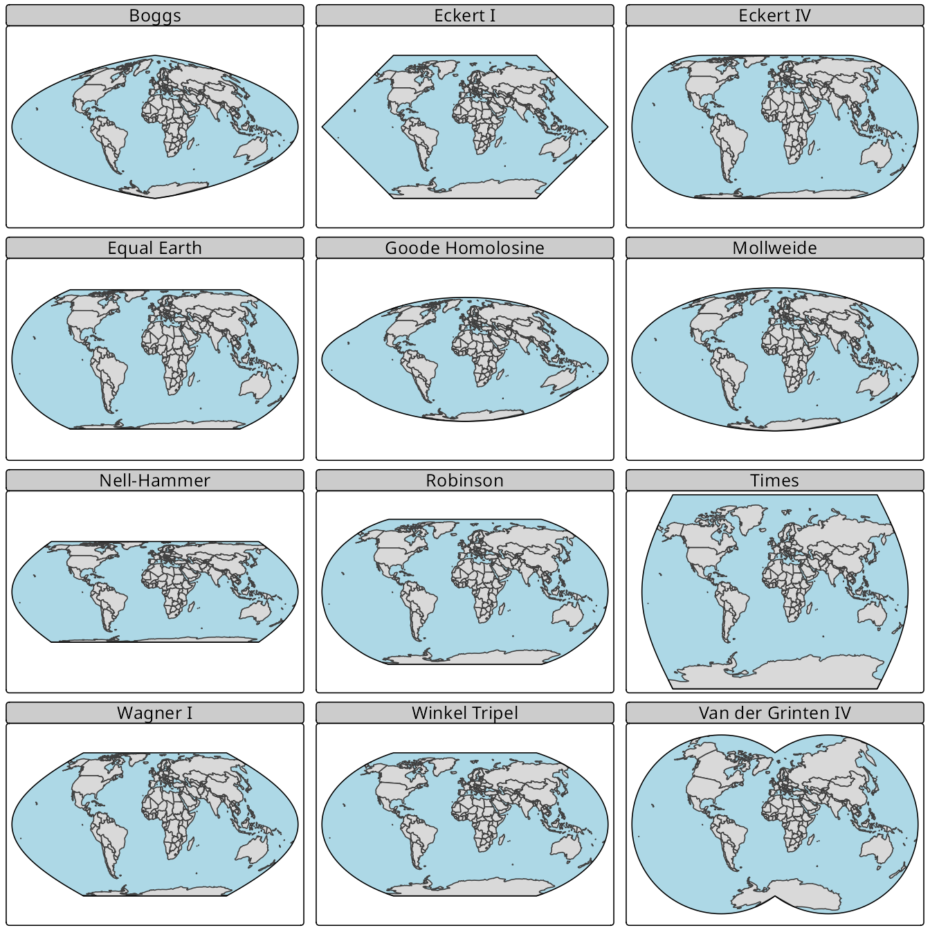
The tmap package also offers several additional features that can be used to customize maps with global projections. For instance, the tm_layout() function has an argument earth_boundary that can be set to TRUE to add a boundary around the Earth. Then, we can also set the bg.color argument to specify the background color of the map, which only applies to the area inside the Earth’s boundary for a given projection (@ @ Figure 13.14).
These features can be used to create more visually appealing maps. They are available to a large set of projections2, some of which are shown in Figure 13.15. You may notice that these projections have not only different visual styles but also different shapes of the Earth’s boundary and focus on preserving different map projection properties.
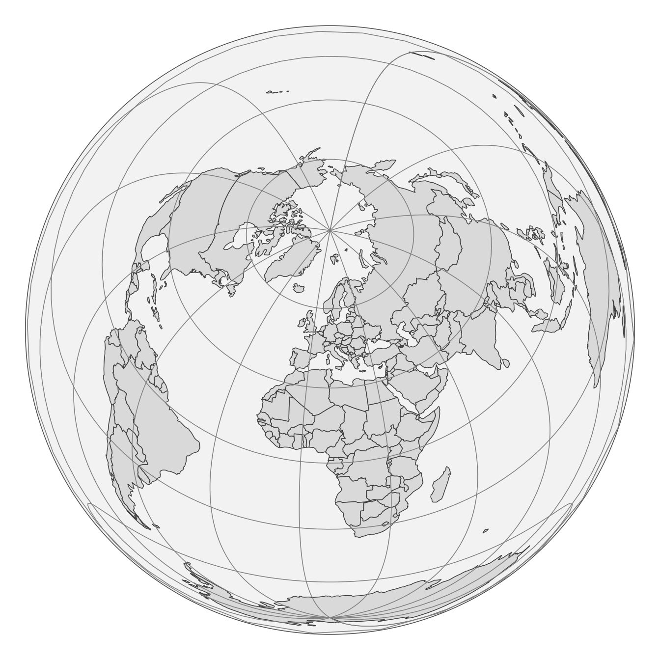
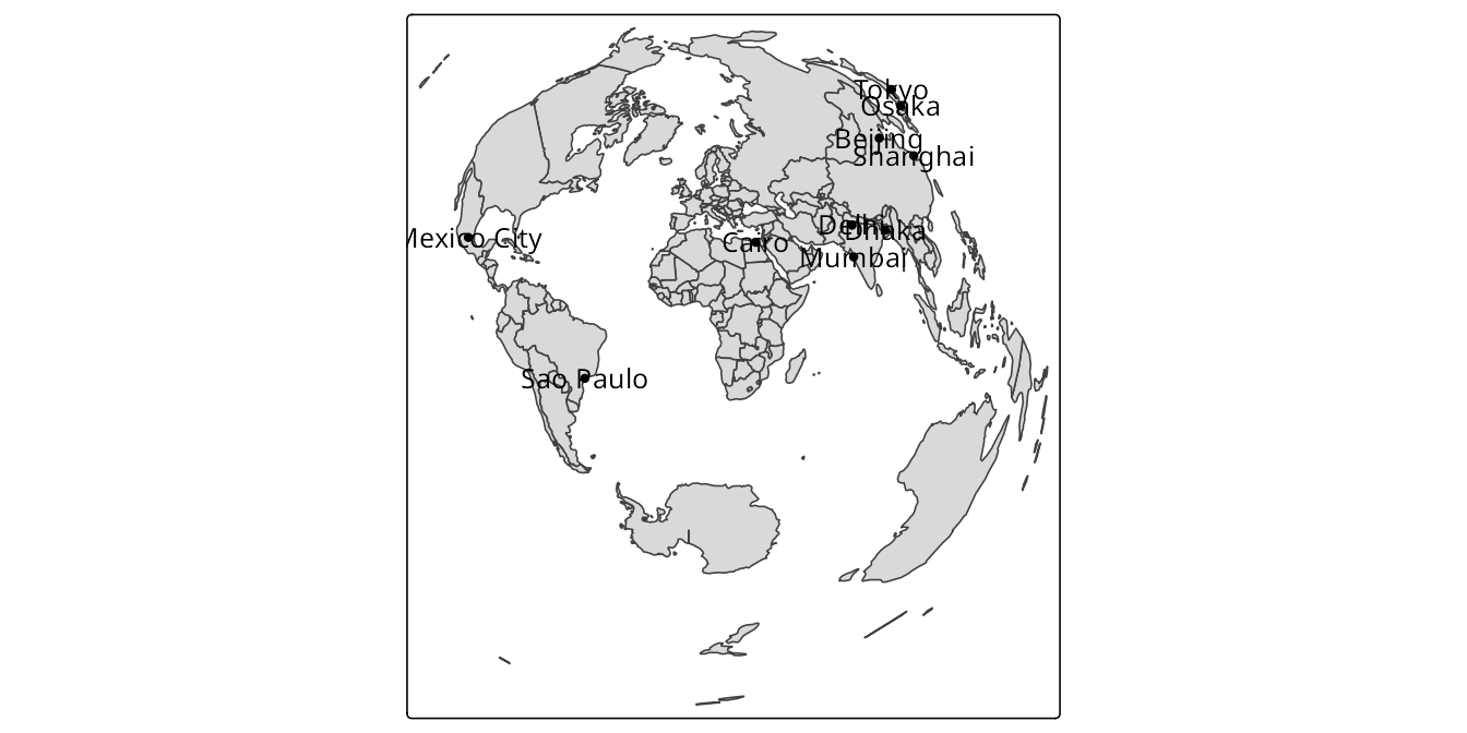
One particular projection that is worth mentioning is the orthographic projection. It is a planar projection that represents the Earth as if it were viewed from space, with the center of the projection at a specific latitude and longitude. We can use the tm_crs() function to apply the orthographic projection with the +proj=ortho argument, and then set the lat_0 and lon_0 parameters to specify the center of the projection. Figure 13.16 shows two examples of the orthographic projection centered on different coordinates: the first one is centered on 30\(^\circ\)N, 0\(^\circ\)E, and the second one is centered on 0\(^\circ\)N/S, 100\(^\circ\)E.
tm +
  tm_graticules(labels.show = FALSE) +
  tm_crs("+proj=ortho +lat_0=30 +lon_0=0", bbox = "FULL")+
  tm_layout(bg.color = "lightblue",
            earth_boundary = TRUE,
            frame = FALSE)
tm +
  tm_graticules(labels.show = FALSE) +
  tm_crs("+proj=ortho +lat_0=0 +lon_0=100", bbox = "FULL")+
  tm_layout(bg.color = "lightblue",
            earth_boundary = TRUE,
            frame = FALSE)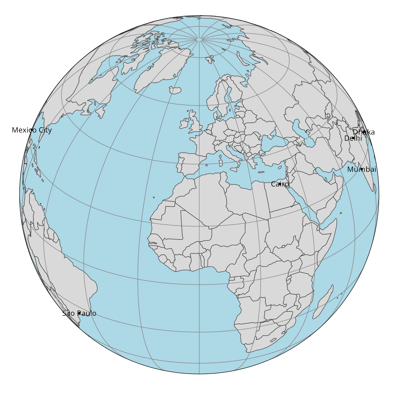
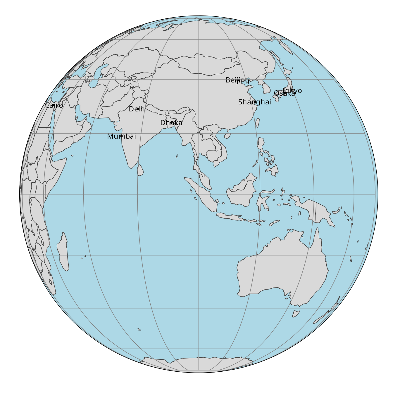
Note
Note that in these examples, the bbox argument is set to "FULL", which means that the whole Earth is displayed – it is useful when the extent of the data is smaller than the whole Earth.
For more details of the first approach, see
?stars::st_warp()and of the second approach, see?stars::st_transform().↩︎Find more projections in the PROJ documentation at https://proj.org/en/stable/operations/projections↩︎