5 Specifying spatial data
At least two aspects need to be specified in order to plot spatial data: the spatial data object itself and the plotting method(s). We cover the former in this chapter and the latter is discussed in the following chapters.
5.1 Shapes and layers
As described in Chapter 2, shape objects can be vector or raster data. We recommend sf objects for vector data and terra objects for raster data1.
In tmap, a shape object needs to be defined with the function tm_shape(). When multiple shape objects are used, each has to be defined in a separate tm_shape() call. This is illustrated in the following example (Figure 5.1).
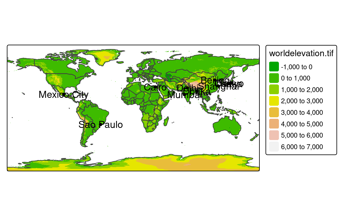
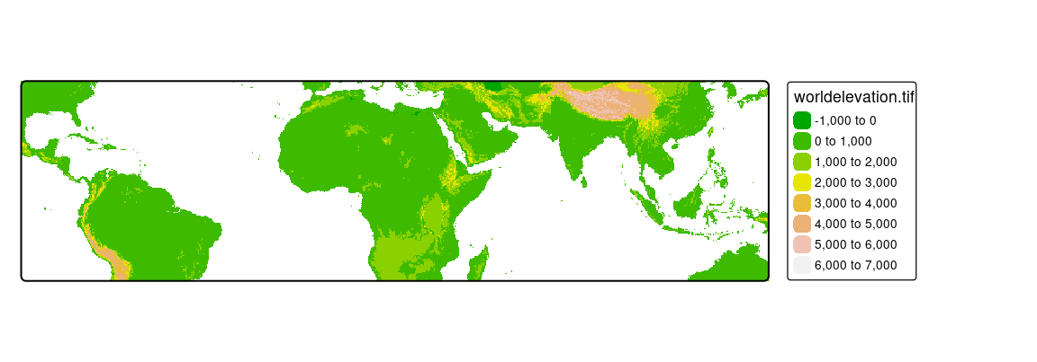
In this example, we use three shapes: worldelevation which is a SpatRaster object containing a layer called "worldelevation", worldvector which is an sf object with country borders, and worldcities – an sf object that contains metropolitan areas of at least 20 million inhabitants.
Each tm_shape() function call is succeeded by one or more layer functions. In the above example, these are tm_raster(), tm_borders(), tm_dots() and tm_text(). We describe layer functions in detail in the next chapter. For this chapter, it is sufficient to know that each layer function call defines how the spatial data specified with tm_shape() is plotted.
Shape objects can be used to plot multiple layers. In the above example, shape object worldcities is used for two layers: tm_dots() and tm_text().
5.2 Shapes hierarchy
The order of the tm_shape() functions’ calls is meaningful. The first tm_shape(), known as the main shape, is not only shown below the following shapes, but also sets the projection and extent of the whole map. In Figure 5.1, the worldelevation object was used as the first shape, and thus the whole map has the projection and extent of this object.
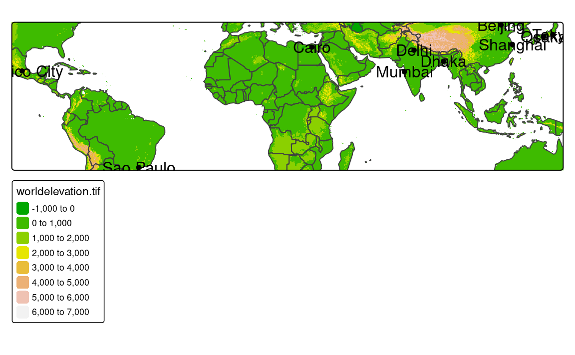
However, we can quickly change the main shape with the is.main argument. In the following example, we set the worldcities object as the main shape, which limits the output map to the point locations in worldcities (Figure 5.2)2.
5.3 Map extent
Another important aspect of mapping, besides projection, is its extent3 – a portion of the area shown in a map. This is not an issue when the extent of our spatial data is the same as we want to show on a map. However, what should we do when the spatial data contains a larger region than we want to present?
Again, we could take two routes. The first one is to preprocess our data before mapping - this can be done with vector clipping (e.g., st_intersection()) and raster cropping (e.g., st_crop()). We would recommend this approach if you plan to work on the smaller data in the other parts of the project. The second route is to specify the map extent in tmap.
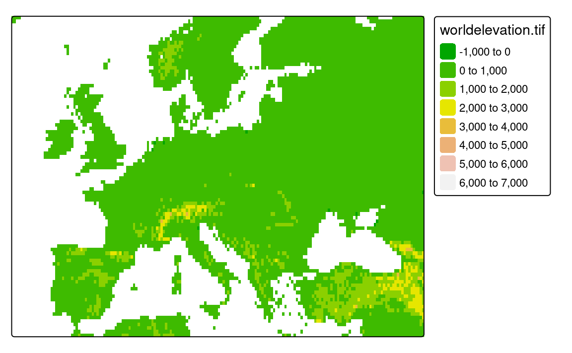
tmap allows specifying map extent using three approaches. The first one is to specify minimum and maximum coordinates in the x and y directions that we want to represent. This can be done with a numeric vector of four values in the order of minimum x, minimum y, maximum x, and maximum y, where all of the coordinates need to be specified in the input data units4 In the following example, we limit our map extent to the rectangular area between x from -15 to 45 and y from 35 to 65 (Figure 5.3).
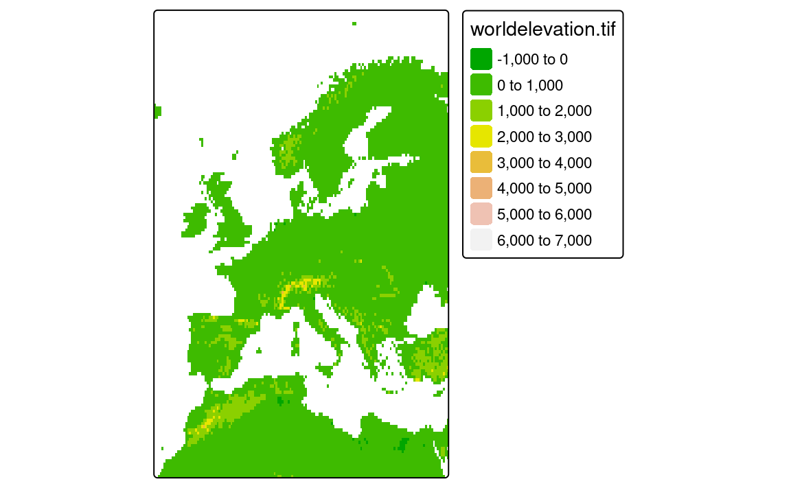
The second approach allows for the map to be set to an extent based on a search query. In the code below, we limit the map extent to the area of "Europe" (Figure 5.4). This approach uses the OpenStreetMap tool called Nominatim to automatically generate minimum and maximum coordinates in the x and y directions based on the provided query.
In the last approach, the map extent is based on another existing spatial object. Figure 5.5 shows the elevation raster data (worldelevation) limited to the outermost coordinates from worldcities.
5.4 Map projection
As we mentioned in the previous section, tmaps use the projection from the main shape. However, we often want to create a map with a different projection, for example, to preserve a specific map property. We can do this in three ways:
- Use a different projection on a map is to reproject the main data before plotting.
- Specify the map projection using the
crsargument oftm_shape(). This argument expects either somecrsobject or a CRS code. - Use a
tm_crs()function.
The next code chunk shows all three ways in which we transform the CRS of the worldvector object to "EPSG:8857" – representing a projection called Equal Earth (Šavrič et al. 2019). The Equal Earth projection is an equal-area pseudocylindrical projection for world maps similar to the non-equal-area Robinson projection (Figure 13.6).
#1
worldvector8857 = st_transform(worldvector, crs = "EPSG:8857")
tm_shape(worldvector8857) +
  tm_polygons()
#2
tm_shape(worldvector, crs = "EPSG:8857") +
  tm_polygons()
#3
tm_shape(worldvector) +
  tm_polygons() +
  tm_crs("EPSG:8857")
The first way requires understanding various R packages, as different spatial objects have different functions for changing the projection. The second way is the most straightforward, but it is important to remember that the crs argument can only be set in the main layer (Section 5.2). The third way is the most flexible, as it allows changing the projection for the whole map. Additionally, the tm_crs() function can automatically determine the projection based on the expected property of the map, e.g., equal area ("area"), equidistant ("distance"), or conformal ("shape"). For example, tm_crs("auto") chooses the projection that best preserves the area of the map (Lambert Azimuthal Equal Area), while tm_crs("auto", property = "shape") chooses the projection that best preserves the shape of the map (Stereographic).
Chapter 13 expands on the topic of map projections. It starts by explaining the basic concepts and then shows how to apply them in tmap.