16 Facets
Facets, also known as small multiples, are a powerful way to visualize multiple variables or values of a single variable in a grid of panels. In other words, they open the possibility of visualizing multiple maps in a single figure. They allow for quick comparison of different variables or values across the same regions or time periods. This chapter not only shows how to define facets in tmap but also how to customize them to make them more informative and appealing.
To demonstrate the use of facets, we will use a few datasets from Slovenia. This includes the borders of Slovenia (slo_borders – just one polygon), the regions of Slovenia (slo_regions – multiple polygons for many variables) and the regions of Slovenia over time (slo_regions_ts – multiple polygons with a time variable representing different years). To simplify the examples, we will subset the slo_regions_ts dataset to include only five years: 2006, 2010, 2014, 2018, and 2022.
16.1 Specifying facets
Facet can be based on data coming from various sources: it can be a set of variables (e.g., columns in an sf object) or a single variable with multiple values.
The first approach is seen below, where we specify multiple variables (c("pop_dens", "gdppercap", "tourism")) from the slo_regions dataset to create facets. Each variable is displayed in its own facet with a separate scale and legend (Figure 16.1). This allows for quick comparison of different variables across the same regions.
tm_shape(slo_regions) +
  tm_polygons(c("pop_dens", "gdppercap", "tourism"))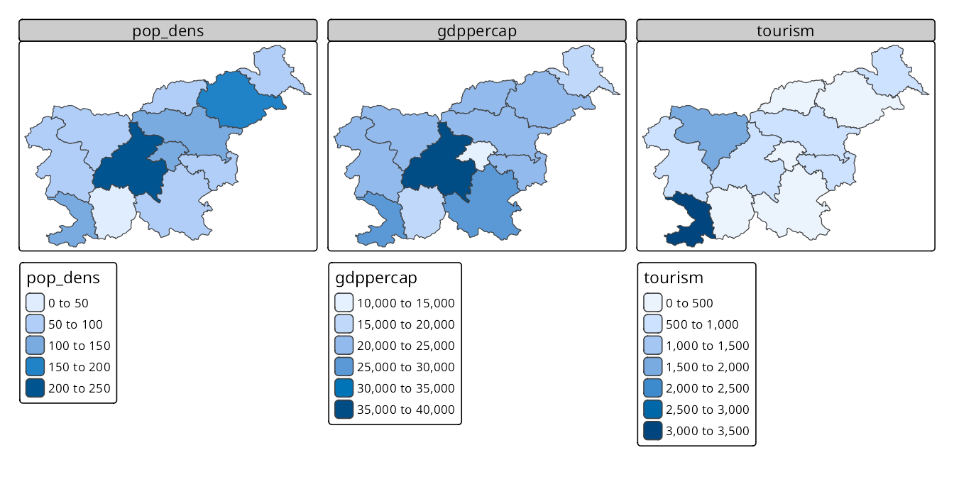
The second approach uses a single variable to create facets, where each facet represents a unique value of that variable. Here, we need to use tm_facets() to specify the faceting variable. This function creates a grid of panels, each showing the data for a specific value of the variable (here "time"), and also allows specifying the layout of the facets (e.g., number of columns) (Figure 16.2). In such cases, all of the facets share the same scale and legend, which is useful, for example, for comparing the same variable across different times.
tm_shape(slo_regions_ts) +
  tm_polygons("gdppercap") +
  tm_facets(by = "time", ncol = 5)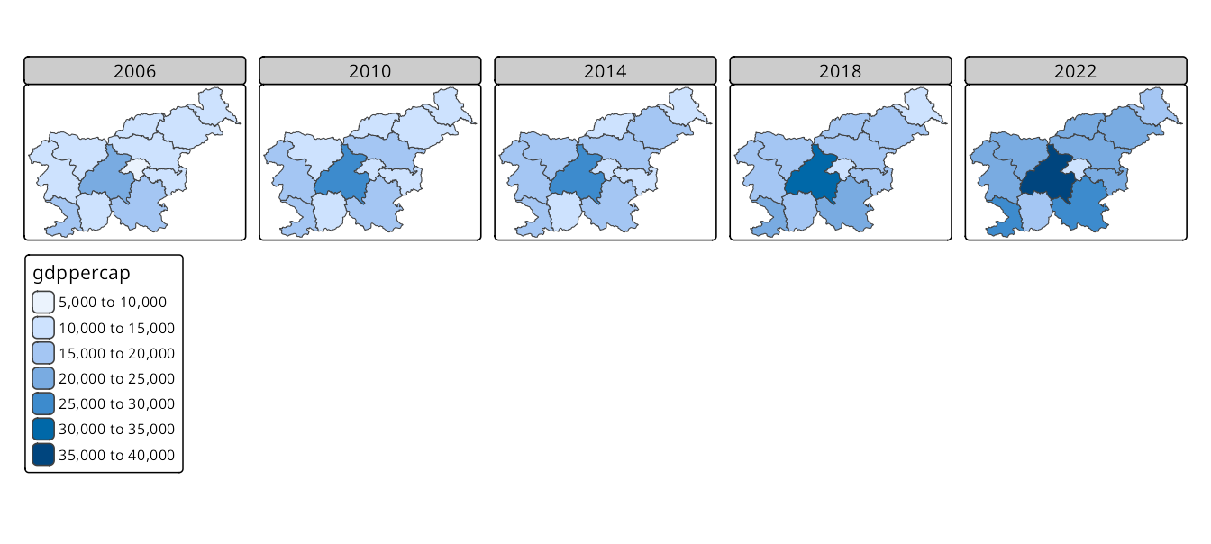
Both approaches can be combined, allowing to create facets for multiple variables over time (Figure 16.3). Here, variables specified as a visual variable (c("pop_dens", "gdppercap", "tourism")) are shown in columns, while the faceting variable is set with tm_facets(by = "time") and presents the data for each year in a separate row.
tm_shape(slo_regions_ts) +
  tm_polygons(c("pop_dens", "gdppercap", "tourism")) +
  tm_facets(by = "time")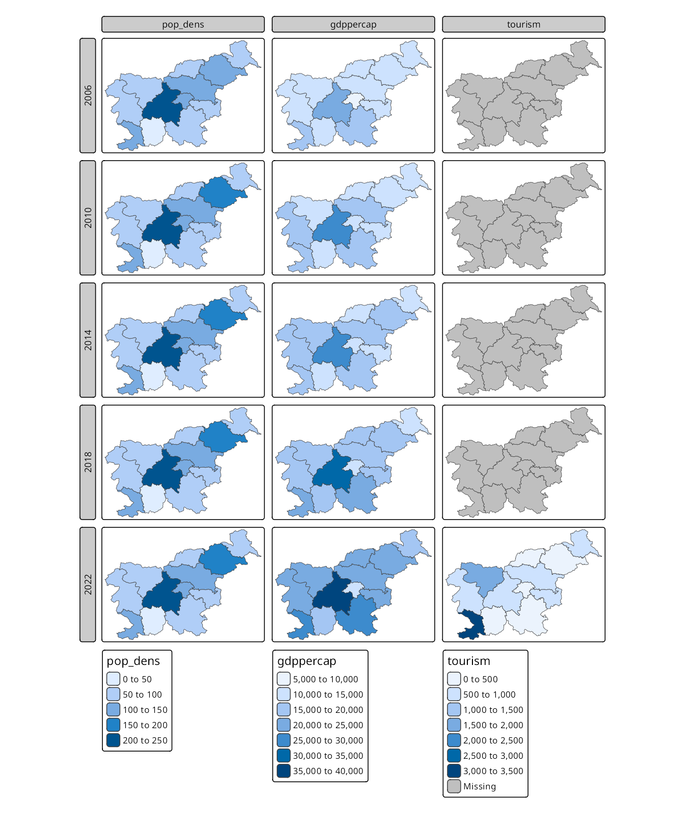
16.2 Importance of layers order for faceting
The placement of the tm_facets() function in the code is crucial for how facets are applied to the map. When presenting multiple layers in a map, the tm_facets() function must be defined after the layer to be faceted.
Moreover, the order of layers is essential when using facets for two reasons:
- The first layer in the map is used to determine the extent of the map.
- Each layer lies on top of the previous one, so the last layer is the one that is in the foreground.
Figure 16.4 has the slo_borders layer first, which means that the borders of Slovenia are drawn first – each facet will have the same extent and the borders will be visible in each facet. Next, the slo_regions_ts layer is added and faceted by the region_group variable. This results in a map where each facet shows the GDP per capita for different region groups with the borders of Slovenia in the background.
tm_shape(slo_borders) +
  tm_borders(lwd = 4) +
  tm_shape(slo_regions) +
  tm_polygons("gdppercap") +
  tm_facets(by = "region_group", nrow = 2)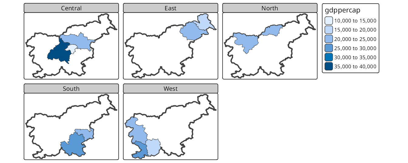
On the other hand, Figure 16.5 has the slo_regions_ts layer first, which means that the GDP per capita is drawn first, and then the borders of Slovenia are added. This results in a map where each facet zooms into a specific region group, showing the GDP per capita for that group.
tm_shape(slo_regions) +
  tm_polygons("gdppercap") +
  tm_facets(by = "region_group", nrow = 2) +
  tm_shape(slo_borders) +
  tm_borders(lwd = 4)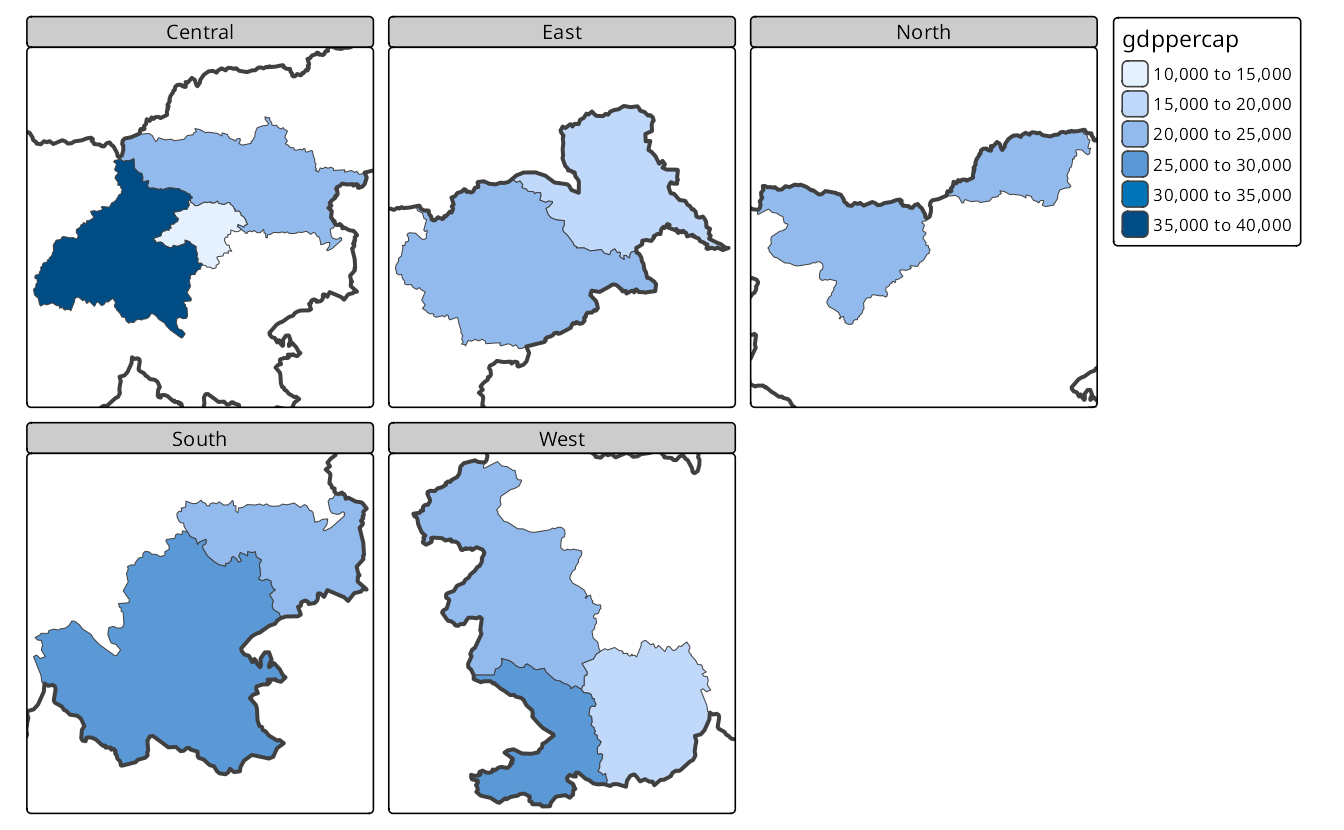
What to do in case we want to keep the borders layer on the top, but also have its extent in every panel? In this case, we may either set the slo_borders layer as a main one (tm_shape(slo_borders, is.main = TRUE); Section 5.2) or set the free.coords argument of tm_facets() to FALSE – then each facet will use the complete extent of the provided slo_regions_ts data.
tm_shape(slo_regions) +
  tm_polygons("gdppercap") +
  tm_facets(by = "region_group", nrow = 2, free.coords = FALSE) +
  tm_shape(slo_borders) +
  tm_borders(lwd = 4)
16.3 Facets types
All of the above examples use the tm_facets() function. This is a general function that can be used to create facets for various types of data. At the same time, tmap provides several specialized functions for creating facets that can be used to create more complex faceting layouts.
The most common ones are:
-
tm_facets_wrap()– creates facets that wrap around the specified variable – it can be thought as a one-dimensional grid of panels -
tm_facets_grid()– creates facets in a two-dimensional grid, where the specified variables define the rows and columns
Figure 16.6 shows how to use tm_facets_wrap() to create facets for the region_group variable, wrapping the panels into two rows. By default, the panels are filled from left to right, and then from top to bottom, but we can change this behavior by setting the byrow argument to FALSE.
tm_shape(slo_borders) +
  tm_borders(lwd = 4) +
  tm_shape(slo_regions) +
  tm_polygons("gdppercap") +
  tm_facets_wrap(by = "region_group", nrow = 2, byrow = FALSE)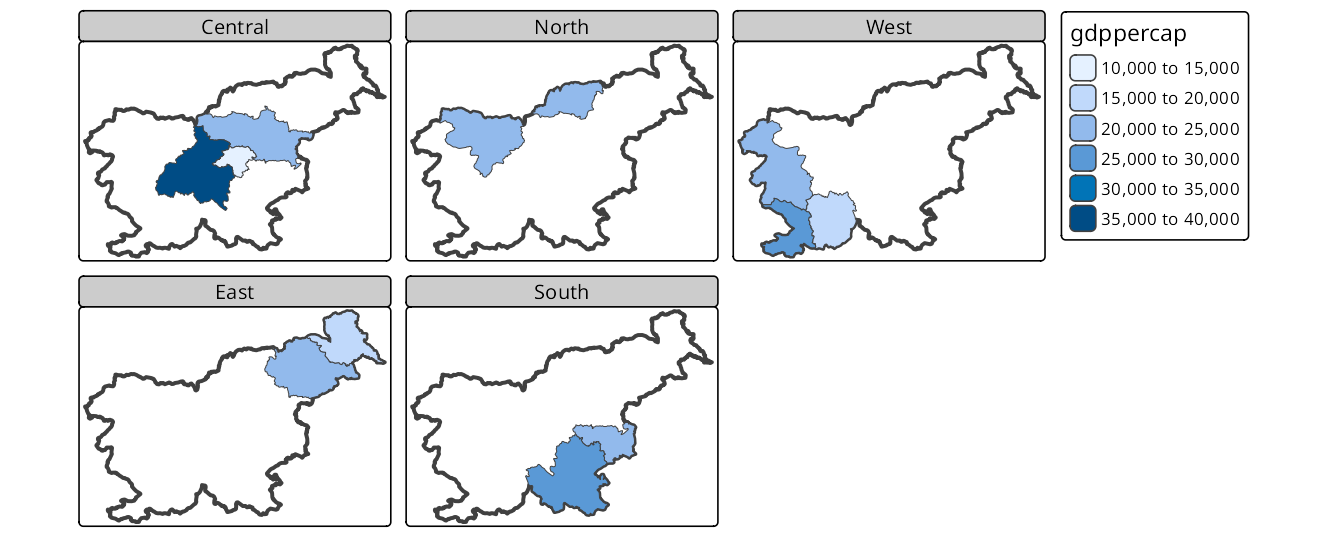
Two-dimensional facets are shown in Figure 16.7, where the region_group variable is used for the rows and the time variable for the columns.
tm_shape(slo_borders) +
  tm_borders(lwd = 4) +
  tm_shape(slo_regions_ts) +
  tm_polygons("gdppercap") +
  tm_facets_grid(rows = "region_group", columns = "time")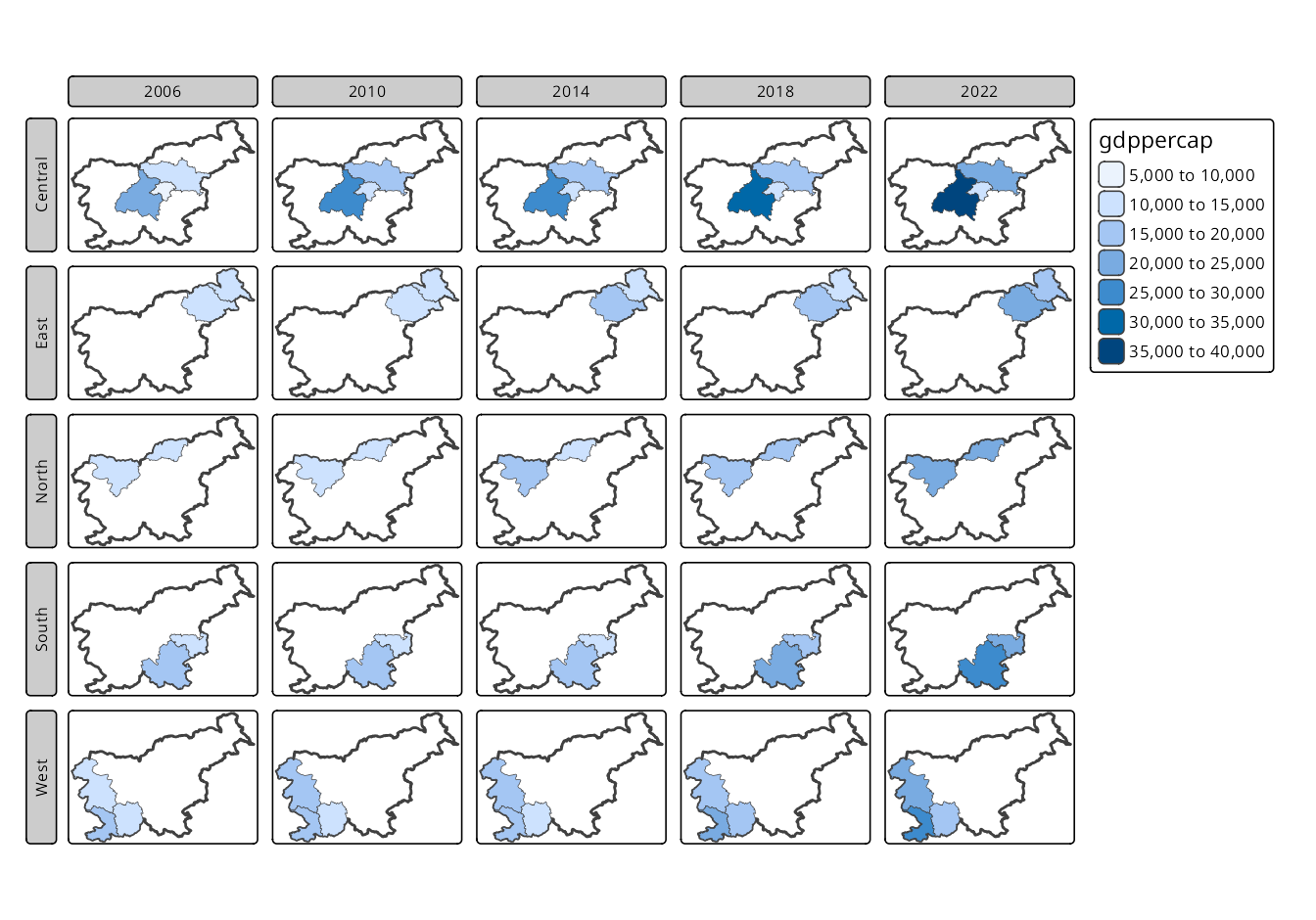
16.4 Customizing facets
Now that we know how to create facets, we can customize them to make them more informative and to focus on the message we want to convey. Often, faceting variables are self-explanatory – we can easily understand what their values mean. However, sometimes, we want to add more information to the facets, such as labels for the axes or titles for the panels.
The labels can be added using the tm_xlab() and tm_ylab() functions (Figure 16.8). By default, they are located on the bottom and left side of the map, but we can change their position using the side argument. Moreover, they maintain a horizontal orientation. This is fine for the x-axis, but not for the y-axis, where we may want to rotate the label to be vertical with the rotation argument. Finally, we could customize their size and distance from the map border to make them more readable using the size and space arguments, respectively.
tm_shape(slo_borders) +
  tm_borders(lwd = 4) +
  tm_shape(slo_regions_ts) +
  tm_polygons("gdppercap") +
  tm_facets_grid(rows = "region_group", columns = "time") +
  tm_xlab("Year", side = "top", size = 2, space = 1) +
  tm_ylab("Region", rotation = 90, size = 2, space = 1)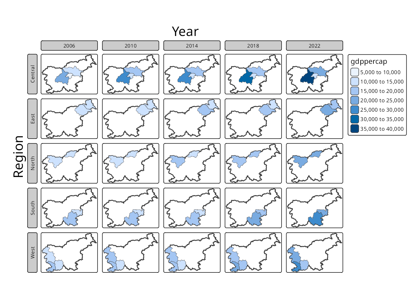
Panel labels can be adjusted using the tm_layout(panel.labels = c(...)) function. To see it in action, we read the slo_tavg raster data, which contains average monthly temperatures in Slovenia.
Next, we create facets for the raster data using tm_facets() and set the number of columns to three – this results in a grid of panels, each showing the average temperature for a specific month. Default layer names are usually not very informative, so we can replace them with more descriptive labels using a vector of labels provided to the panel.labels argument of the tm_layout() function, e.g., panel.labels = c(1:12) (Figure 16.9).
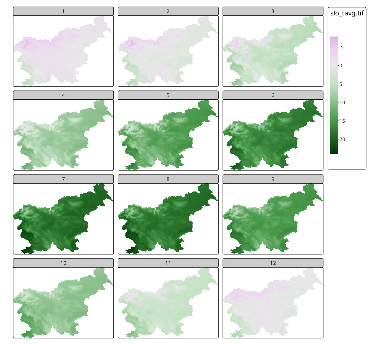
Note that in the above example only one legend is shown and it is shared across all panels. This allows for easy comparison of the values across different months, e.g., we can see that the average temperature in January is much lower than in July.
On the other hand, we may be interested in comparing the spatial patterns of average temperatures across different months rather than their values. To do that, we need to create independent legends for each panel – we should set the col.free argument of tm_raster() to TRUE (Figure 16.10). In the example below, we also customize the map further by updating the color scale to use the “viridis” palette, removing the title from the legend and adding a title to the map, improving the panel labels, and adjusting the inner margins of the facets to make them more readable.
tm_shape(slo_tavg) +
  tm_raster(
    col.scale = tm_scale_continuous(values = "viridis"),
    col.legend = tm_legend(title = "", position = c("LEFT", "BOTTOM")),
    col.free = TRUE) +
  tm_facets(ncol = 3) +
  tm_layout(panel.labels = c(1:12),
            inner.margins = c(0.02, 0.2, 0.02, 0.02)) +
tm_title("Average monthly temperature in Slovenia") 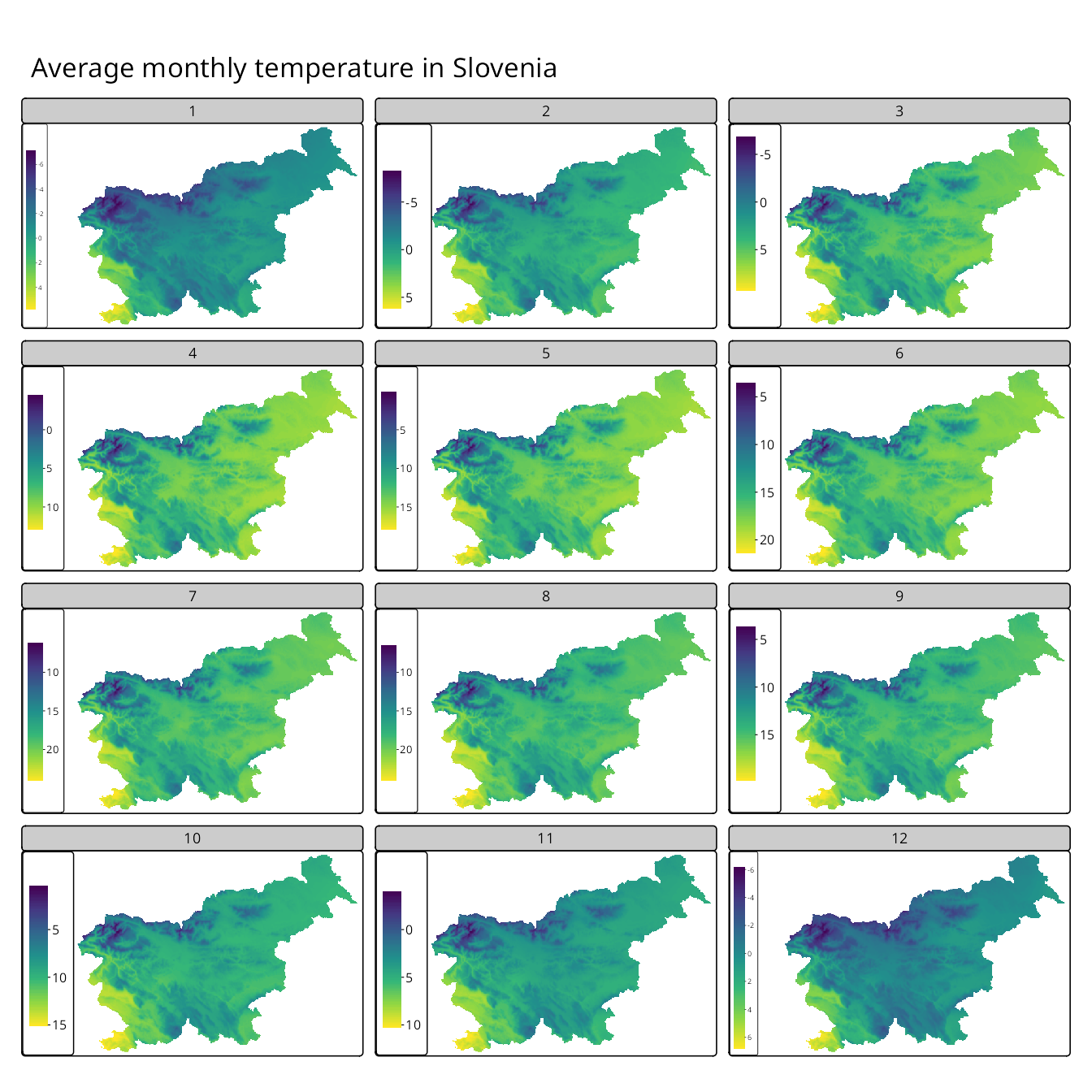
Each visual variable (e.g., col, size, shape) has a related argument with the .free suffix, e.g., col.free, size.free, shape.free. These arguments are used to control whether the scales for the visual variable are applied freely across facets or are shared. For example, col.free = TRUE means that each facet has its own color scale, while col.free = FALSE means that all facets share the same color scale.
The .free arguments can also be used to control the scales for each facet dimension with a vector of logical values. For example, col.free = c(TRUE, FALSE) means that the color scale is applied freely across rows of facets, but shared across columns.
16.5 Facets with raster and vector data
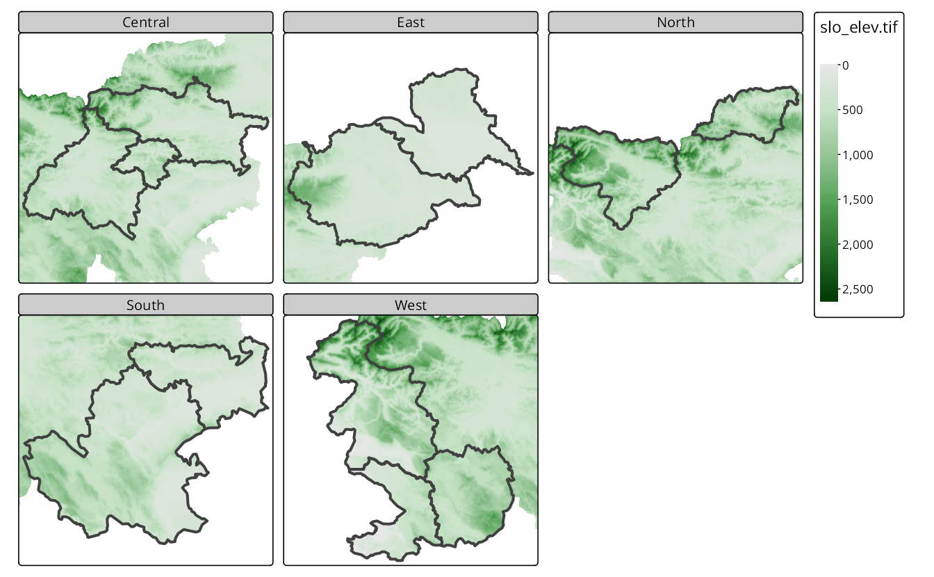
Figure 16.11 shows how to combine raster and vector data in facets. In this example, we use the slo_elev raster data, which contains elevation data for Slovenia, and the slo_regions vector data, which includes the borders of the regions in Slovenia. To display the elevation data for each region group, we must first specify the raster data and then use the vector data as the main layer (is.main = TRUE in tm_shape()). Next, we can use tm_facets() to create facets for the region_group variable.
slo_elev = rast("data/slovenia/slo_elev.tif")
tm_shape(slo_elev) +
  tm_raster(col.scale = tm_scale_continuous()) +
  tm_shape(slo_regions, is.main = TRUE) +
  tm_borders(lwd = 4) +
  tm_facets(by = "region_group", free.coords = TRUE)