3 tmap in a nutshell
The tmap package creates thematic maps with great flexibility. It accepts spatial data in various formats – shape objects (Section 3.1) and next, the data can be used to create simple, quick maps (Section 3.2) and more complex and expandable maps (Section 3.3). Additionally, with tmap it is possible to create facet maps (Section 3.4) and map animations (Section 3.5). Finally, tmap has an interactive mode (Section 3.6) that allows users to zoom in and out, pan the map, or click on map objects to get more information – this can be done without any additional code. The goal of this chapter is to provide a brief overview of the main tmap features.
3.1 Shape objects
As we established in Chapter 2, spatial data comes from various file formats related to two main data models – vector and raster. There are also several spatial object classes in R, for example, sf from the sf package for vector data, SpatRaster from the terra package, and stars from stars for raster data and spatial data cubes. Additionally, packages such as sp or raster offer their own classes, and this abundance of spatial object classes can be generally overwhelming. Gladly, tmap can work with all of the above objects – it treats all supported spatial data classes as so-called shape objects.
For example, we read the slo_cities.gpkg file containing several point locations representing cities and towns in Slovenia into a new object, slo_cities. The slo_cities object is a shape object.
.
3.2 Quick maps
The tmap package offers two distinct ways to create maps: a quick and a regular one. The first approach, using the qtm() function, could be handy for data exploration. It works even if we provide any shape object – in that case, only the geometry is plotted. Figure 3.1 (a) shows a visualization of the geometries from the slo_cities.
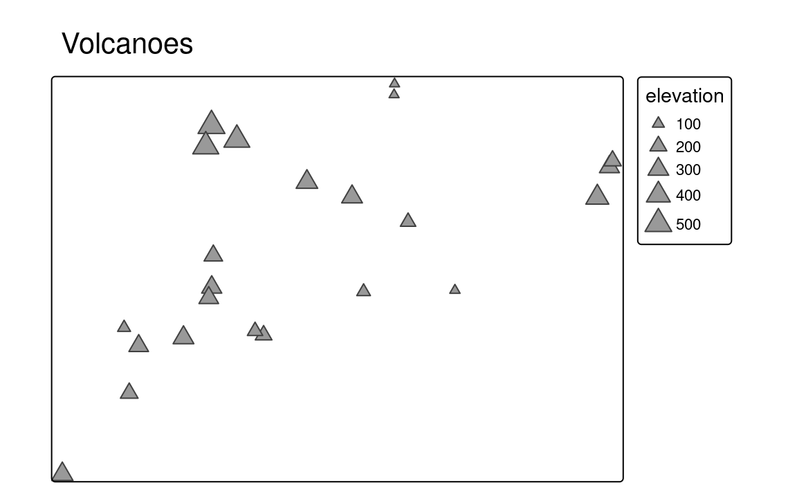
qtm(slo_cities)The qtm() function customizes many map elements for the provided shape object. For example, we can change the shapes of the points in slo_cities, make their sizes related to the the "population" argument, and add a title (Figure 3.1 (b)).
qtm(slo_cities, shape = 24, size = "population", title = "Cities")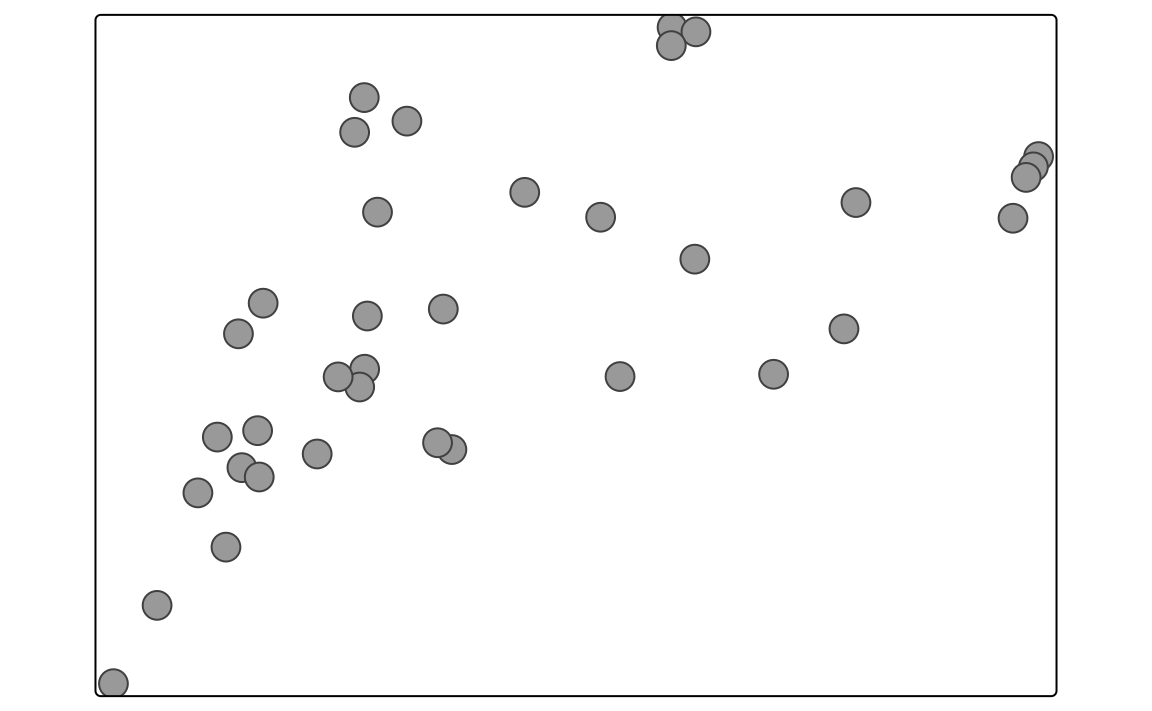
qtm() function.
The qtm() function is a quick way to create maps, but it has some limitations. It supports only one shape object at a time and does not allow for much customization.
3.3 Regular maps
For most applications, we recommend using the regular mapping approach. This approach operates on many functions with the tm_ prefix that we call one after another with the + operator. We call these functions tmap elements. The first element always1 is tm_shape(), which specifies the input shape object. Next, map layers (e.g., tm_polygons() or tm_symbols()), additional map components (e.g., tm_compass() or tm_scalebar()), and overall layout options can be customized.
The last example in Section 3.2 can be reproduced with the regular map approach using the following code.
tm_shape(slo_cities) +
  tm_symbols(shape = 24, size = "population") +
  tm_title("Cities")
Here, we specify the input data (our shape object) with tm_shape(), visual variables (also known as aesthetics) of map layers with tm_symbols(), and the map title with tm_title().
The tmap package has a number of possible map layers, but the most prominent ones are tm_polygons(), tm_symbols(), tm_lines(), tm_raster(), and tm_text() (Chapter 6). Overall, most visual variables of map layers can be assigned in two main ways. First, they accept a fixed, constant value, for instance, shape = 24, which sets the symbols’ shapes to triangles. Second, it is also possible to provide a variable name, for example, size = "population". This plots each point with a size based on the population attribute from the slo_cities object and automatically adds a related map legend.
The tm_shape() function and one or more of the following map layers create a group together. In other words, map layers are related only to the preceding tm_shape() call. One map can have several groups. Let’s see how many groups can be used by reading some additional datasets – the slo_elev raster with elevation data of Slovenia, the slo_borders polygon with the country borders, and the slo_railroads lines contain a railroad network for this country.
Look at the following example and try to guess how many groups it has, and how many layers exist for each group (Figure 3.2).
tm_shape(slo_elev) +
  tm_raster(col.scale = tm_scale(values = "geyser"),
            col.legend = tm_legend(title = "Elevation (m asl)")) +
  tm_shape(slo_borders) +
  tm_borders() +
  tm_shape(slo_railroads) +
  tm_lines(lwd = "track_width",
           lwd.legend = tm_legend(show = FALSE)) +
  tm_shape(slo_cities) +
  tm_symbols(shape = 24, size = "population",
             size.legend = tm_legend(title = "Population")) +
  tm_title("Slovenia") +
  tm_layout(bg.color = "grey95")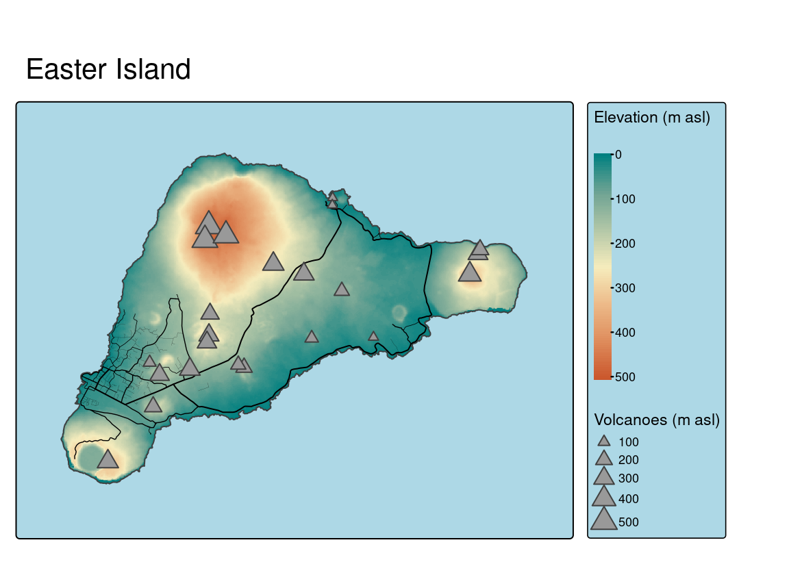
The correct answer is four groups, all with just one layer. Each group is put on top of the previous one – tmap uses a layered approach. The first group represents elevation data with a continuous color scale style, a color palette called "geyser", and a legend title. The second group shows the borders of Slovenia with the default aesthetics, while the third group presents the railroad network (the slo_railroads object), with each line’s width based on the values from the "track_width" column, but with a legend hidden. The last group is similar to our previous example with fixed symbol shapes and sizes related to the "elevation" attribute, but also with the legend title instead of the map title. Additionally, we use the tm_title() function to add a map title and tm_layout() to modify the general appearance of the map. You can also notice that we can control scales of various visual variables, such as color, size, or width, with the tm_scale_*() function and customize legends with the tm_legend() function.
Often, maps also have map components, such as graticule lines, north arrow, scale bar, or map credits (Figure 3.3). They help map readers understand the location or extent of the input data and provide some ancillary information. The tmap package offers a set of functions for additional map elements. The tm_graticules() function draws latitude and longitude graticules and adds their labels. It also uses the layered approach, and thus, the lines are drawn either below or above the shape objects, depending on the position of this function in the code. In our example below, tm_graticules() is used after all of the map groups, and that is why the graticule lines are put on the top of the spatial data. We can also use tm_compass() to create a north arrow, tm_scalebar() to add a scale bar, and tm_credits() to add a text annotation representing credits or acknowledgments. The location of all these three elements on the map is, by default, automatically determined. It, however, can be adjusted with the position argument – see an example of its use in the tm_compass() function below. Moreover, it is possible to add any type of manual legend with tm_add_legend(). It includes simple legends below, such as the "Railroads" legend element, that is only represented by a single black line and a related label, but more complex custom legends with several elements are also possible.
my_map = tm_shape(slo_elev) +
  tm_raster(col.scale = tm_scale(values = "geyser"),
            col.legend = tm_legend(title = "Elevation (m asl)")) +
  tm_shape(slo_borders) +
  tm_borders() +
  tm_shape(slo_railroads) +
  tm_lines(lwd = "track_width",
           lwd.legend = tm_legend(show = FALSE)) +
  tm_shape(slo_cities) +
  tm_symbols(shape = 24, size = "population",
             size.legend = tm_legend(title = "Population")) +
  tm_graticules() +
  tm_compass(position = c("right", "top")) +
  tm_scalebar() +
  tm_credits("Author, Year") +
  tm_add_legend(type = "lines", col = "black", labels = "Railroads") +
  tm_title("Slovenia") +
  tm_layout(bg.color = "grey95")
Maps created with tmap can be saved as R objects. This is a useful feature that allows the use of the same map in a few places in a code, modify existing tmap objects by adding additional tmap elements, or save these objects to files.
my_map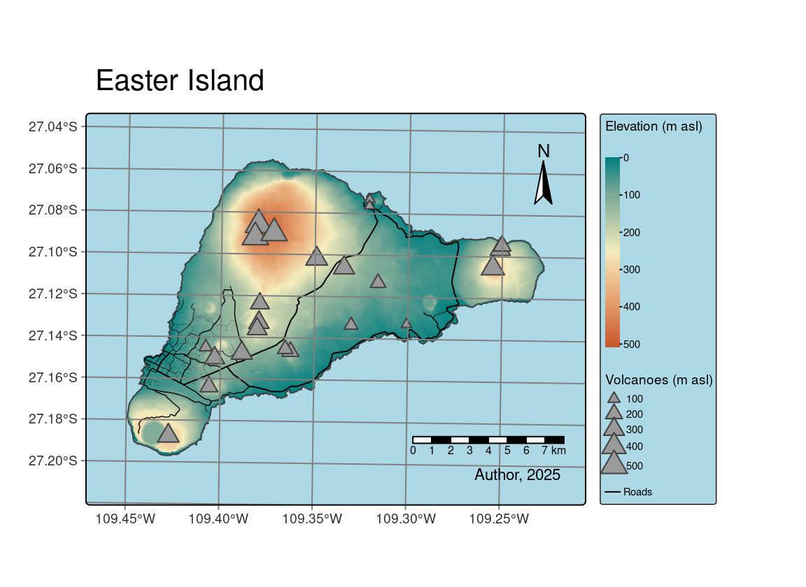
All of these building blocks of tmap maps are explained in more detail in chapters from Chapter 5 to Chapter 12.
3.4 Facets
The tmap package makes the creation of facet maps, also known as small multiples, possible. In such maps, the same data is visualized in several panels, each showing a different subset of the data. The panels may represent different variables, time periods, or spatial extents.
The slo_regions object contains the administrative regions of Slovenia with their names, population density (gdppercap), GDP per capita (gdppercap), region group name (region_group), and other attributes. One way to visualize this data as facets is to specify selected columns as visual variables in the map layer function (e.g., tm_polygons()) (Figure 3.4).
slo_regions = read_sf("data/slovenia/slo_regions.gpkg")
tm_shape(slo_regions) +
  tm_polygons(fill = c("pop_dens", "gdppercap", "region_group"))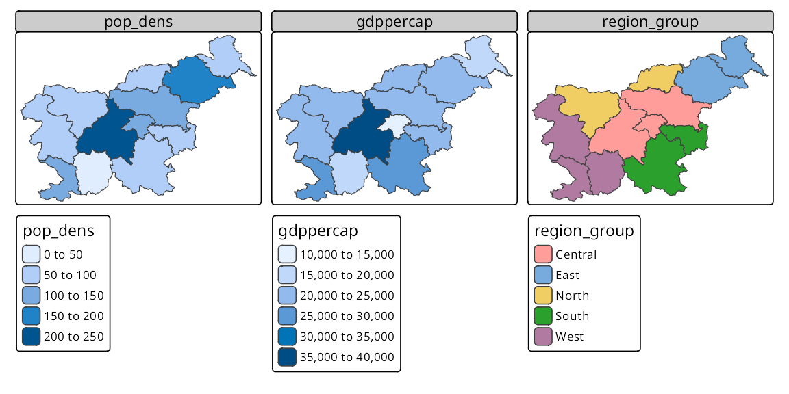
Another possible approach is to use the tm_facets() function. Let’s illustrate it with the slo_regions_ts object containing the same variables as slo_regions but for many years (time column). Figure 3.5 shows a facet map with the GDP per capita, specified with tm_polygons(), and visualized in separate panels for each year as defined by the tm_facets() function.
slo_regions_ts = read_sf("data/slovenia/slo_regions_ts.gpkg")
tm_shape(slo_regions_ts) +
  tm_polygons("gdppercap") +
  tm_facets(by = "time", ncol = 5)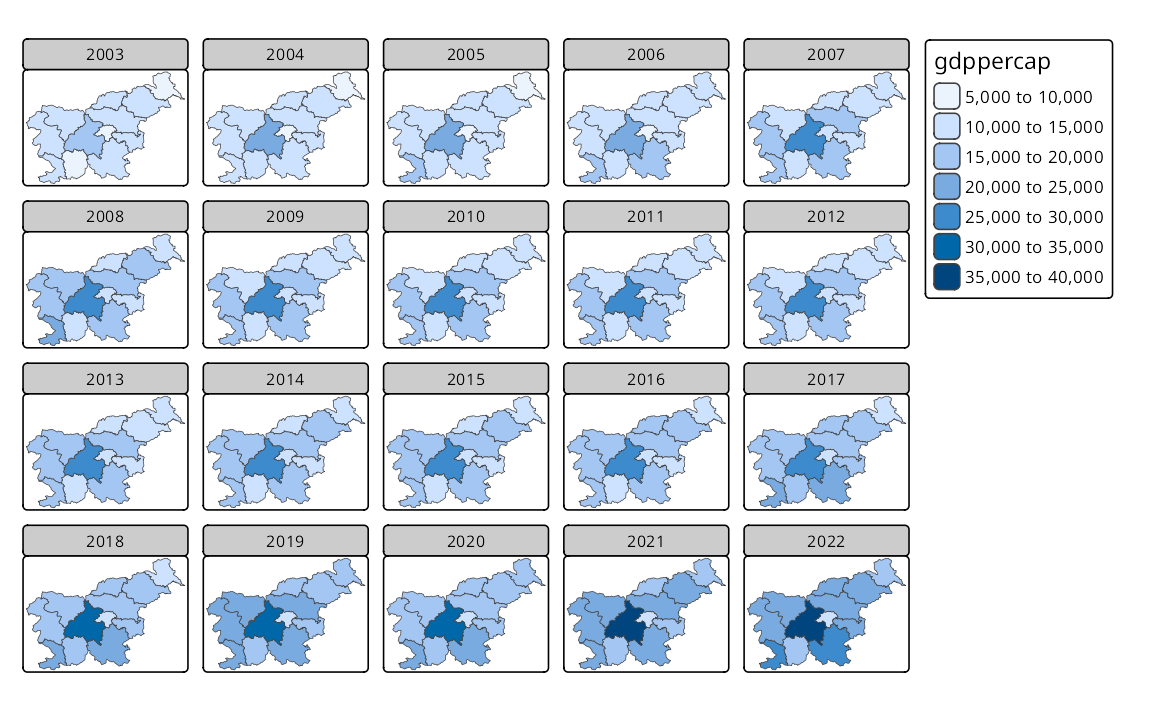
Facet maps can be used for vector and raster data, their extents can be adjusted, and they can be further customized with additional labels. This is a topic of the Chapter 16.
3.5 Animations
Figure 3.6 shows an animated map with the GDP per capita visualized for each year. Animations in tmap are created similarly to the facet maps, but instead of using the tm_facets() function, we use the tm_animate() function. It defines the variable that is used to create the animation, in this case, the time column from the slo_regions_ts object.
slo_regions_ts = read_sf("data/slovenia/slo_regions_ts.gpkg")
tm_shape(slo_regions_ts) +
  tm_polygons("gdppercap") +
  tm_animate(frames = "time")
This function stitches together the map layers for each value of the time variable, creating a smooth transition between them. We can customize its speed and if it should loop or not with the fps and play arguments, respectively. Animations can be used for both vector and raster data and then saved as GIF or video files using the tmap_animation() function. Chapter 17 expands on this topic and shows how to create more complex animations, such as animated maps with facets.
3.6 Map modes
Each map created with tmap can be viewed in a few map modes, including the "plot" and "view" modes. The "plot" mode is used by default and creates static maps similar to those shown before in this chapter. This mode supports almost all of tmap’s features, and it is recommended, for example, for scientific publications or printing.
The second mode, "view", creates interactive maps. They can be zoomed in and out or panned, allow for changing background tiles (basemaps), or click on map objects to get some additional information. This mode has, however, some constraints and limitations compared to "plot", for example, the legend cannot be fully customized, and some additional map elements are not supported.
It is important to highlight that both modes can be used with the same tmap code. Therefore, there is no need to create two separate sets of code for static and interactive use. The tmap_mode() function can be used to switch from one mode to the other2.
tmap_mode("view")
#> ℹ tmap mode set to "view".
The above line of code just changes the mode – it does not return anything except a message. Now, if we want to use this mode, we need to either write a new tmap code or provide some existing tmap object, such as my_map.
my_mapOur result now is the interactive map (Figure 3.7). It shows our spatial data using aesthetics similar to Figure 3.3 but allows us to zoom in and out or move the map. We also can select a basemap or click on any line and point to get some related information.
To go back to the "plot" mode, we need to use the tmap_mode() function again – map not shown.
tmap_mode("plot")
my_map
More information about the interactive "view" mode and how to customize its outputs is in Chapter 18.
Almost always…↩︎
Map modes can also be changed globally using
tmap_options()or switched usingttm().↩︎